
Sensitivity/Uncertainty Multimedia Modeling Module
User´s Guidance
G. M. Gelston, M. A. Pelton, K. J. Castleton, B. L. Hoopes, R. Y. Taira, P. W. Eslinger, G. Whelan, P. D. MeyerSUMMARY
The Framework for Risk Analysis in Multimedia Environmental Systems (FRAMES) software is currently designed for deterministic environmental and human health impact models. The Sensitivity/Uncertainty Multimedia Modeling Module (SUM3) software product was designed to allow a statistical analysis using the existing deterministic models available in FRAMES. SUM3 is an available option under the Sensitivity/Uncertainty Module in FRAMES. SUM3 randomly samples input variables and preserves associated output values in an external file available to the user for evaluation. This enables the user to calculate deterministic values with variable inputs, producing a statistical distribution of results. A typical application of the uncertainty analysis is to indicate relative conservatism of the deterministic result. This document serves as guidance for Version 2 of SUM3.
Although SUM3 was originally developed as a sensitivity/uncertainty tool for use with the Multimedia Environmental Pollutant Assessment System (MEPAS©), it is not restricted to MEPAS© models. SUM3 can now be used with other deterministic environmental models through the FRAMES software package with other available tools, such as the Generation II (GENII) software system, which is a Hanford environmental dosimetry system. Within FRAMES, SUM3 allows users to conduct a sensitivity and/or uncertainty analysis to understand the influence and importance of variability/uncertainty input parameters on constituent flux, concentration, and human health impacts. The sensitivity analysis can identify the key parameters that dominate overall uncertainty. Statistical methods used in SUM3 are based on Monte Carlo sampling using Latin Hypercube random numbers. This file contains the cumulative distribution function (CDF) data and can be graphically displayed through the FRAMES Viewer option.
This document takes users through a step-by-step process for setting up a statistical analysis, running SUM3 software, and interpreting results. Examples of input screens and result files are provided along with a full example case analysis.
Contents
1.0 Introduction
2.0 Using FRAMES Sensitivity/Uncertainty Module
3.0 Selecting Sampling Variables of Interest
4.0 Entering Statistical Parameters
4.1 Distribution
- 4.1.1 Uniform
4.1.2 Log Uniform
4.1.3 Normal
4.1.4 Log Normal
4.1.5 Exponential
4.1.6 Triangular
4.1.7 Gamma
4.1.8 Beta
4.1.9 Weibull
4.1.10 Logistic
4.1.11 User Defined
4.3 Equation
5.0 Selecting Output Variables of Interest
6.0 Running Sensitivity Uncertainty Module And SUM3
6.1 Status Screen
6.2 SUM3 Sampling Technique
7.0 Interpreting Results
8.0 Example Illustrating Application of Sensitivity Uncertainty Module
8.1 Introduction
8.2 Background
8.3 Predictive and Comparative Assessments
8.4 Predictive Assessment
- 8.4.1 Calibration Process
8.4.2 Calibration Parameters and Results
8.4.3 Probabilistic Human-Health Risk Assessment for Ethylbenzene, Toluene, and Xylene
- 8.5.1 Comparative Assessment Scenarios
8.5.2 Deterministic Assessment (Scenarios 1 and 2)
8.5.3 Probabilistic Human-Health Risk Assessment for Benzene and TCE (Scenario 3)
Tables
Table 8.1 1994 Monitored Ground Water Concentrations for Ethylbenzene, Toluene, and Xylene at MW-2 and MW-4
Table 8.2 Calibrated Hydrogeologic and Hydrodynamic Parameters
Table 8.3 Exposure Parameters
Table 8.4 Stochastic Saturated Zone Parameters
Table 8.5 Stochastic Constituent Flux Data in Predictive Assessment
Table 8.6 Stochastic Parameters in Comparative Assessment
1.0 Introduction
This uncertainty analysis provides a quantitative estimate of the range of model outputs resulting from uncertainties in the structure of a software model or inputs to a model. If an analysis is carried out in the appropriate way, the range will likely contain the true value (or values) the model seeks to predict. This analysis can also be extended to identify the input parameters that contribute most to overall uncertainty, so priorities can be set for work aimed at reducing uncertainty. The sensitivity analysis allows users to identify the parameters that impact results the most. If uncertainty estimates are to be made meaningful and practical, the analysis must be carried out systematically, with due regard to the purpose of the model, quality of data, and the nature of application. Uncertainty in model predictions can arise from a number of sources, including specification of problem, formulation of conceptual models, formulation of computational models, estimation of parameter values, and calculation, interpretation and documentation of results. Of these sources, only uncertainties resulting from the estimation of parameter values can be quantified in a straightforward way by applying a statistical approach to deterministic models.
This document serves as guidance for the Sensitivity/Uncertainty Multimedia Modeling Module (SUM3) Version 2. SUM3 is currently an option under the Sensitivity/Uncertainty Module in Framework for Risk Analysis in Multimedia Environmental Systems (FRAMES). FRAMES software is designed for deterministic models. Therefore, the SUM3 software product was designed to allow a statistical analysis using deterministic models. SUM3 will randomly sample input variables and preserve associated output values in external file available to user for evaluation. effect is calculating deterministic values with variable inputs producing a statistical distribution of results. A typical application of uncertainty analysis is to indicate relative conservatism of deterministic result. Note within FRAMES software, SUM3 model is located in Sensitivity/Uncertainty Module.
Although SUM3 was originally developed as a sensitivity/uncertainty tool for use with the Multimedia Environmental Pollutant Assessment System (MEPAS©), it is not restricted to use with MEPAS© models. SUM3 can now be used with other deterministic environmental models through FRAMES. Within FRAMES, SUM3 allows users to conduct a sensitivity and uncertainty analysis of an input parameter´s variability/uncertainty on constituent flux, concentration, and human health impacts. The results of this analysis can be used to identify the key parameters that dominate overall uncertainty. Statistical methods used in SUM3 are based on Monte Carlo sampling using Latin Hypercube random numbers. This file contains the Cumulative Distribution Function (CDF) data and can be graphically displayed through the FRAMES Viewer option.
This document takes users through a step-by-step process for setting up, running, and interpreting results from a sensitivity/uncertainty analysis simulation. Examples of user interface screens and results files are provided along with a full example case analysis.
2.0 Using FRAMES Sensitivity/Uncertainty Module
The following section guides users through the use of the Sensitivity/Uncertainty (S/U) Module option in the FRAMES user interface. There are four steps to starting the S/U Module: before using the S/U Module, connecting the S/U Module, choosing the SUM3 model and opening the SUM3 user interface.
Before using the S/U Module:- First set up the deterministic FRAMES analysis (See FRAMES Tutorial), entering a value for each parameter requested.
- Run the deterministic model to ensure there are not errors in base case.
- There should be green lights on all module icons prior to running the S/U Module, with the exception of text or chart viewers.
- Drag and drop a single S/U Module icon onto the FRAMES conceptual model screen. The S/U Module Icon is a bell curve on a green background.
- Using the right-click-and-drag feature of FRAMES, connect the S/U Module icon to each deterministic module icon containing the input variable of interest. Note that the connection path starts at the deterministic module icon and goes to the S/U Module icon. For example, two vadose zone icons and a saturated zone icon can be connected to the S/U module icon, thereby allowing all input and outputs produced by those modules to be available for selection in the SUM3 user interface.
- Shift-Click on S/U Module icon and choose ´General Info´ option.
- From the FRAMES General Info screen, choose ´Sensitivity/Uncertainty Multimedia Modeling Module.´ Available statistical models are listed in the left column, and a description and contact information for highlighted models is displayed in the right column.
- Give the S/U Module icon a Label
- Click OK button
Opening the SUM3 Model User Interface:
- Shift-click on the S/U Module icon and choose ´User Input´ option. This starts the SUM3 user interface.
- From the SUM3 User Interface, users are able to:
- select variables of interest
- choose a distribution for variables of interest
- enter correlation information to describe dependencies between variables
- enter an equation to describe dependencies between two or more variables.
- select output values of interest.
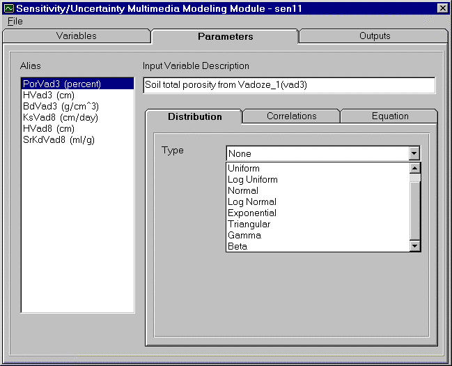
There are three main tabs in the SUM3 user interface: Variables, Parameters, and Outputs. Figure 2.4 illustrates user interface for FRAMES. The Variables tab allows users to select variables of interest. The Parameters tab allows users to describe and relate variables through distributions, correlation, and equations. The Outputs tab allows users to select output values of interest. The following sections describe each tab and its use in more detail.
3.0 Selecting Sampling Variables of Interest
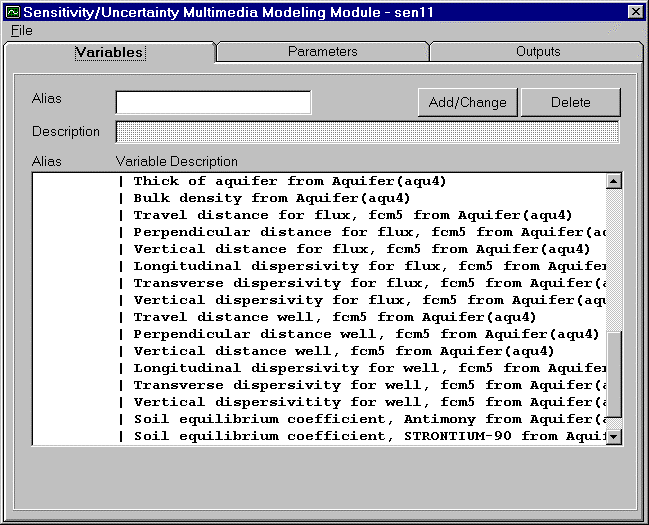
The Variables tab enables users to specify stochastic parameters that are to be randomly sampled and varied. A variable list is provided for users with a description that is consistent with descriptions given in the deterministic module´s input screen. This list of variables is derived from all possible stochastic parameters found in all deterministic modules connected to the S/U Module icon. The description provides users with a variable name and an associated module name (both the module name given by the user and the FRAMES icon name are displayed). Figure 3.1 demonstrates a portion of the listing of stochastic parameters from two vadose zone modules and a saturated zone module that have been connected to the S/U Module icon. A scroll bar is provided on the far right of the listing to enable the user to move through the list when it is longer than the window length.
Adding Alias: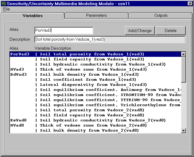
In order to reduce this list to just those parameters the user wishes to vary, the user is asked to provide a unique alias for each parameter of interest. A parameter of interest may be one that is given a distribution, correlation, or used in equation to describe another parameter of interest. To add alias, click on the white entry box to the right of the word "Alias." The alias should be one word (numbers or letters) and is limited to eight (8) digits. Capitalization is preserved but is not used to distinguish between aliases, and the underscore symbol ( _ ) is not allowed. After typing the alias, click Add button to enter alias into the variable list. The variable description list will display alias to the far left with a line ( | ) separating the alias from the description. This alias will be used to create a selection list for distributions, correlation, and equations.
Changing Alias:
To change alias, the user must first delete the old alias then add in the new alias. Following are the instructions given for deleting the alias. The user should remove the alias from all distributions and equations before selecting the alias to be deleted from the variables screen. A warning will appear if any correlation or equation dependencies exist. To add a new alias follow the guidance given for adding an alias.
Deleting Alias:
To delete the alias, the alia must first be removed from all parameter dependencies. The user must first delete any correlation and/or equation where the alias has been assigned. A Delete button is provided in the variables tab to remove a variable from the selection list. A warning will appear if any correlation or equation dependencies exist. By removing a variable from thevariable list, the variable will no longer be available for distributions, correlation, or equations. This allows users to reduce listing to only those currently of interest.
4.0 Entering Statistical Parameters
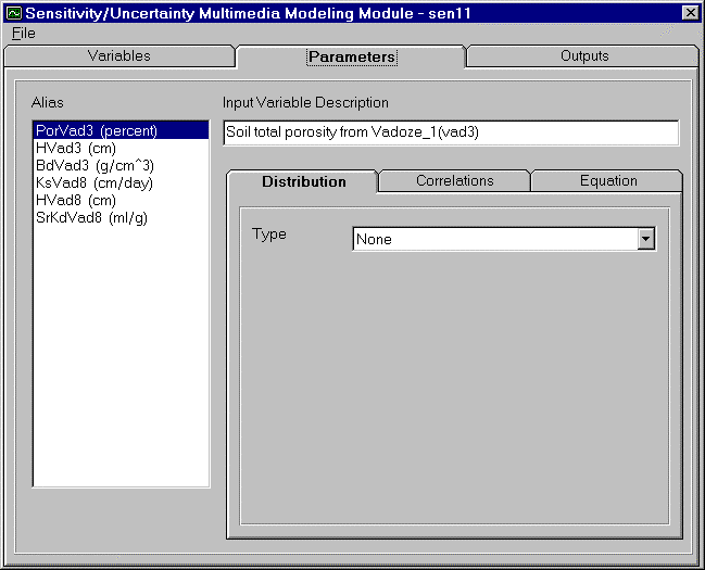
The Parameters Tab enables the user to describe variables of interest. There are three options for describing variables statistically. Figure 4.1 demonstrates the Parameters Tab and three sub-tabs options found within the distribution, correlation, and equation. There are several combinations of these options to aid users in describing variables of interest. Some combinations available to users are:
- giving variable a statistical distribution only,
- giving variable a statistical distribution and correlating to another variable of interest,
- giving variable a statistical distribution and using in equation to describe another variable, and
- using an equation to describe variable.
4.1 Distribution
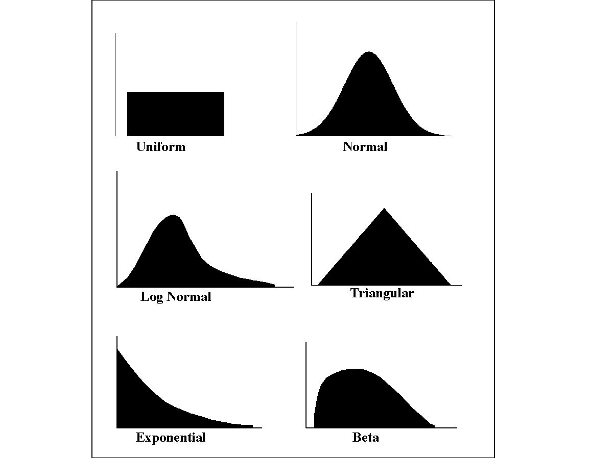
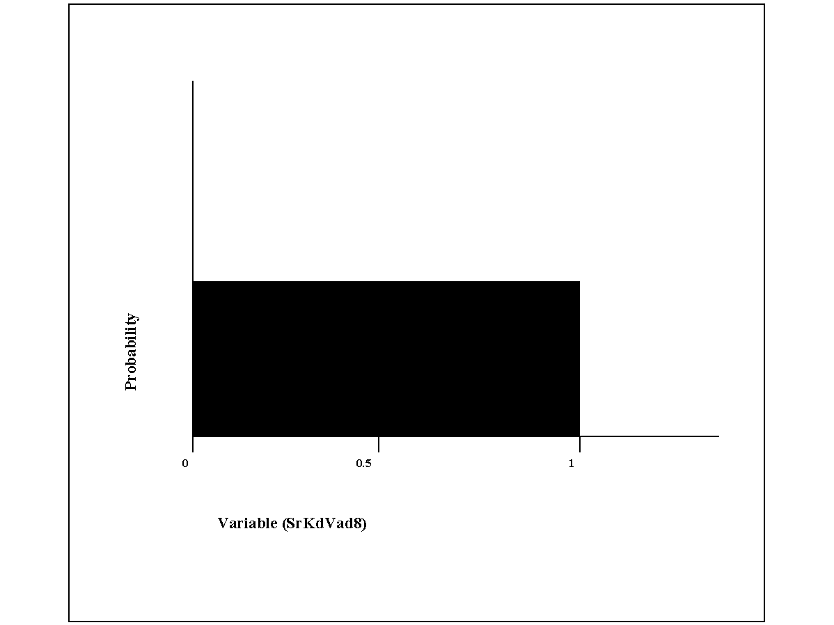
To assign a distribution to a variable, the user must first have assigned a variable (to learn how to assign variables, go to Section 3.0 Selecting Sampling Variables of Interest). Distributions available in SUM3 are: Uniform, Log Uniform, Normal, and Log Normal (Exponential, Triangular, Gamma, Beta, Weibull and Logistic distributions are not available in this version of SUM3). Figure 4.2 gives the example shape for several of the distributions. Each distribution will be discussed in this section. Figure 4.3 shows the dropdown menu of distribution types available in SUM3. The listing of available variable aliases, with their default units, is given in a selection listing on the far left side of the screen. The variable description for the highlighted distribution is given at the top of the screen. The user will be given the option to select the preferred units for distribution input parameters after a specific distribution is selected. SUM3 will convert all units to default units before initiating the simulation.
Selecting a distribution
Click the arrow to the far left of the ´Type´ box located on the distribution tab. This will bring down a selection list. The user can select the distribution type. The user will be given the opportunity to enter the statistical input necessary for the selected distribution. When the distribution parameters are entered, they are preserved specifically for the distribution type.
4.1.1 Uniform
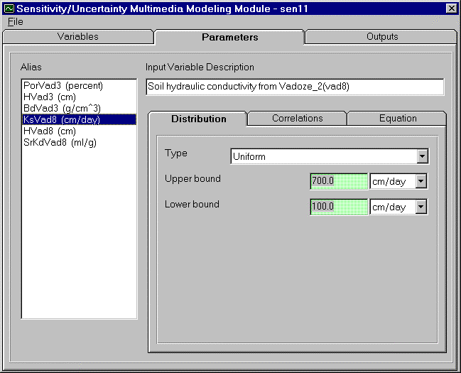
For a uniform distribution all values between minimum value and maximum value are equally likely to be sampled. Figure 4.4 illustrates a uniform distribution. In this example distribution, the variable is soil hydraulic conductivity from second vadose zone. The variable is estimated to be somewhere between 100 cm/day and 700 cm/day. All values between 100 and 700 are equally likely to be selected for each simulation. Figure 4.5 is a view of the input screen for a uniform distribution, where the upper and lower bounds are entered in linear space. Clicking to the right of the units box will activate a selection listing of units. The user can select units for the upper and lower bounds. Note that the user should be careful to adjust both the upper and the lower bounds to the appropriate units to ensure consistency.
4.1.2 Log Uniform
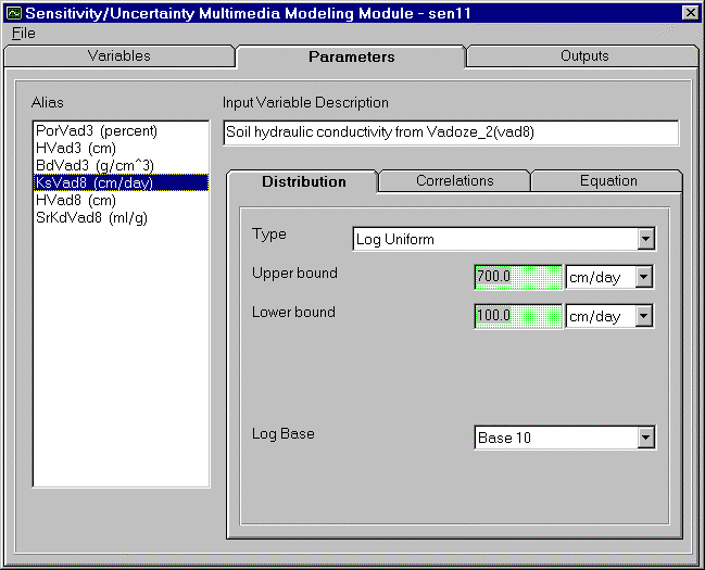
The Log Uniform distribution is like the Uniform Distribution in that all values between the lower and upper bounds are equally as likely to be selected. The additional feature of the Log Uniform distribution is the ability to sample data in Log space or E space. The upper bound and lower bound, however, are entered in linear space. Figure 4.6 illustrates the input screen for the Log Uniform distribution. This screen is similar to the uniform screen, with the addition of the Log Base selection option at the bottom of the tab screen. To choose the Base, click the arrow to the right of the Log Base box. A selection listing will be displayed. Select the Base for the distribution.
4.1.3 Normal
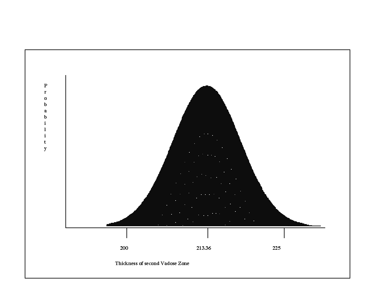
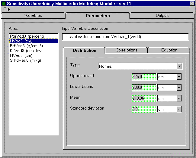
The Normal distribution is the most used distribution in probability theory because it describes many natural phenomena and is useful in describing uncertain variables. This distribution, shown in Figure 4.7, is often described as a bell curve. There are several assumptions common to a normal distribution. First, there is a mean, (i.e. some value of the variable is most likely). Second, the value is symmetrical about the mean, and the uncertain variable could as likely be above the mean as it could be below it. And finally, the uncertain variable is more likely to be in the vicinity of the mean than farther away (i.e. 68% of values are within 1 standard deviation from the mean). Figure 4.7 illustrates a normal distribution for the thickness of the second vadose Zone. In this example, the mean of the distribution is 213.36 cm with a lower bound of 200 cm and an upper bound of 225 cm. The standard deviation for this distribution is given as 5 cm. Figure 4.8 displays the input screen for the normal distribution, where bounds, mean and standard deviation are entered.
4.1.4 Log Normal
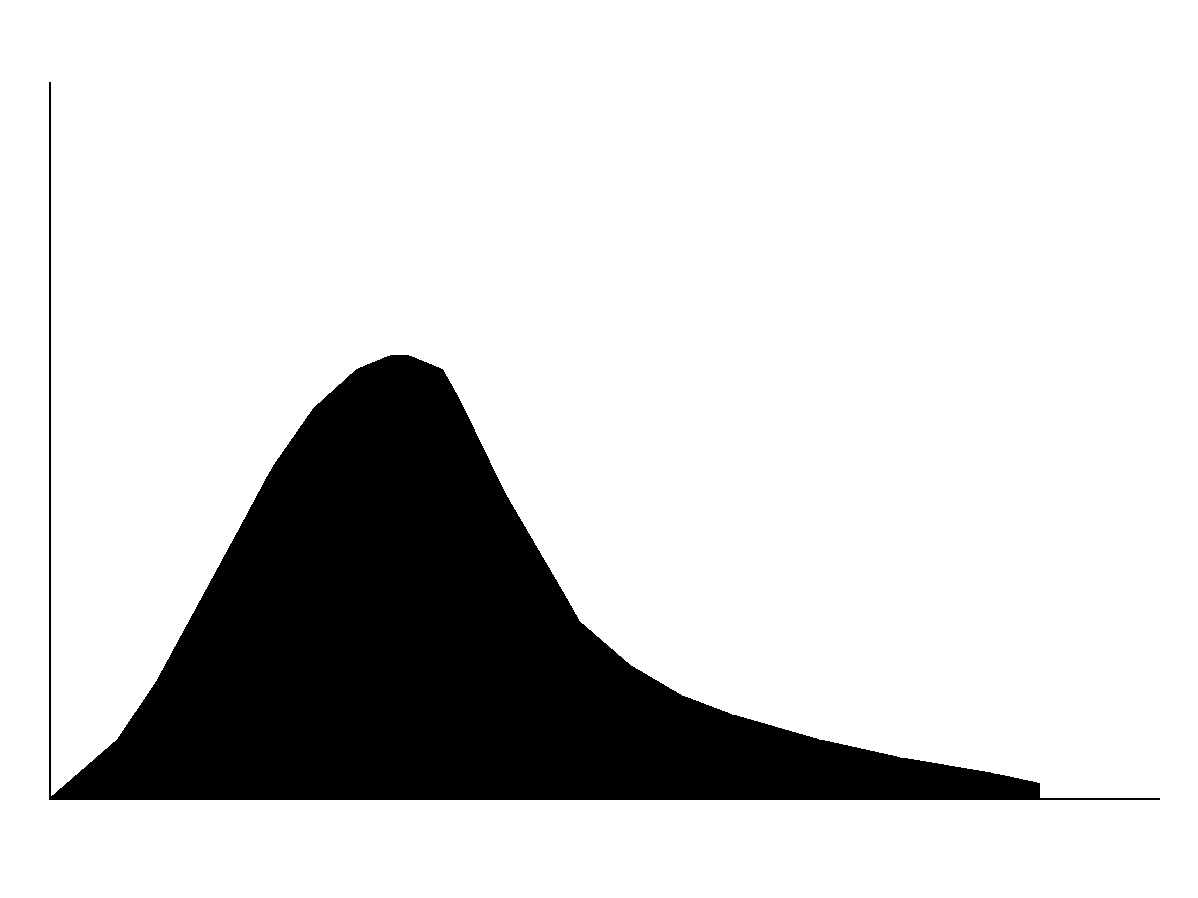
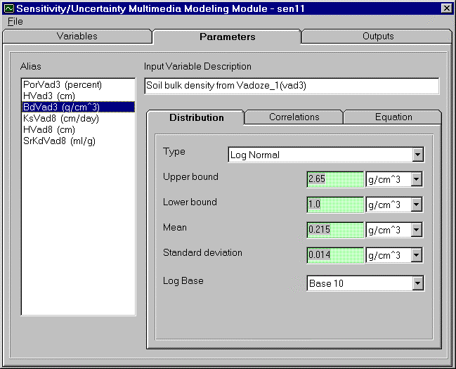
The Log Normal distribution is widely used when most of the values occur near minimum value, or are positively skewed. Figure 4.9 depicts a Log Normal distribution, in linear space, for the soil bulk density from vadose zone one with a lower bound of 1 g/cm3 and an upper bound of 2.65 g/cm3. The mean and standard deviation for the Log Normal distribution should be calculated in log space. For this example, the mean is 0.215 gm/cm3 and the standard deviation is 0.014 g/cm3. There are some assumptions common to a normal distribution. The variable cannot go below zero and the natural Logarithm of the variable is a normal distribution. Figure 4.10 demonstrates the input screen for the Log Normal distribution. Required parameters are the upper bound, lower bound, mean, standard deviation, and Log Base. Upper and lower bounds are expected in linear space. The Mean and Standard Deviation are expected in Log space. There are two choices for the Base available--Base 10 and Base E. To choose the Base, click the arrow to the right of the Log Base box. A selection listing will be displayed. Select the Base for the distribution.
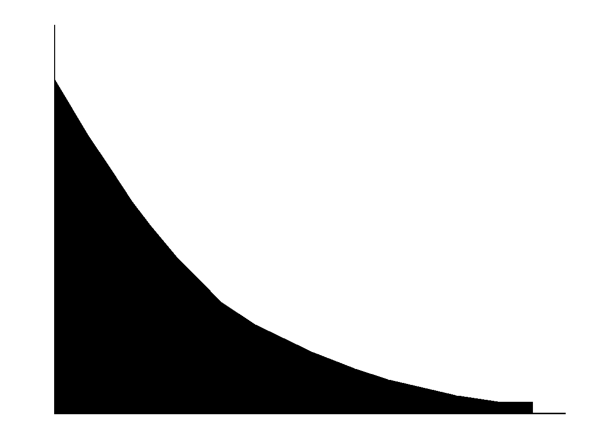
4.1.5 Exponential
The Exponential distribution is widely used to describe events recurring at random in time, such as the time between arrivals at a service booth or the decay of a radionuclide over time. The Exponential distribution has a memoryless property. This important characteristic allows the distribution to have the effect of timelessness. Therefore, the future lifetime of a given parameter has an identical distribution, regardless of when it occurred. Figure 4.11 is the exponential distribution for the radioactive decay of strontium-90.
This distribution is not available in Version 2 of SUM3.
4.1.6 Triangular
To describe the Triangular distribution, the minimum, maximum and most likely values to occur need to be known. This information is often gathered from records on similar events. Figure 4.12 is a triangular distribution.
This distribution is not available in Version 2 of SUM3.
4.1.7 Gamma
The Gamma distribution applies to a wide-range of physical quantities. Environmentally, it is used in precipitation quantities or meteorological processes to represent pollutant concentrations.
This distribution is not available in Version 2 of SUM3.
4.1.8 Beta
The Beta distribution allows for flexibility over a fixed range. A common use of this distribution is to describe empirical data and predict random behavior of percentages and fractions.
This distribution is not available in Version 2 of SUM3.
4.1.9 Weibull
The Weibull distribution is widely used in the field of life phenomena, as the distribution of the lifetime of some object, particularly when the "weakest link" model is appropriate for that object. The "weakest link" model can be described as an instance when an object consists of many parts, but the object experiences failures when any one of its parts fail. Under these types of conditions, it has been shown (both theoretically and empirically) that the Weibull distribution provides a close approximation of the distribution of the lifetime of that object. Weibull distributions can also be used to represent various physical quantities such as wind speed.
This distribution is not available in Version 2 of SUM3.
4.1.10 Logistic
A growth distribution can be described by the Logistic distribution. This distribution may be used to describe the size of a population or individual, expressed as a function of variable time or to describe chemical reactions.
This distribution is not available in Version 2 of SUM3.
4.1.11 User Defined
This distribution is not available in Version 2 of SUM3.
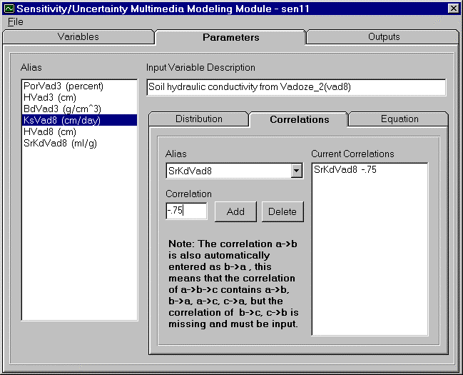
4.2 Correlation
To assign a correlation to a set of variables, the user must first have assigned variables aliases (to learn how to assign go to Section 3.0 Selecting Sampling Variables of Interest). A correlation option is also available in SUM3 to account for dependencies (correlation) between two parameters. The correlation of two variables allows users to ensure the preservation of a relationship between variables. A correlation parameter is a ratio of one variable to another. Therefore, a correlation parameter can range from -1 to +1. A correlation of -1 represents a strong negative correlation, meaning that one variable increases while the second variable decreases. A correlation of +1 represents a strong positive correlation, meaning that one variable increases while the second variable increases. Likewise, a correlation of 0 implies no correlation between variables. Figure 4.13 illustrates the input screen for the variable correlation.
Assign a correlation
To assign a correlation, highlight the first variable to be correlated from the listing on the left of the screen. Then click the arrow on the box on the correlation tab. Select the second variable from the drop down listing. Enter a correlation value in the space provided and click add button. The second variable and the associated correlation will be displayed in the Current Correlation box on the left.
A correlation from variable A to variable B will automatically be entered as a correlation between variable B to variable A. This means, if a variable sequence A->B->C is assigned by the user, then the correlation A->B, B->C, B->A, and C->B are all assigned, however, correlation A->C is not automatically assigned.
Deleting a correlation
To delete a correlation, highlight the first variable to be correlated from the listing on the left of the screen. Then click the arrow on the box on the correlation tab. Select the second variable from the drop down listing. "Confirm correlation to be deleted" appears in the Current Correlation box to the left. Then click the Delete button.
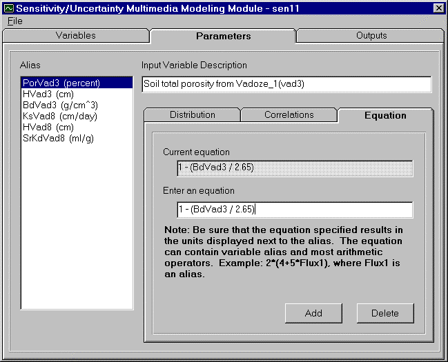
4.3 Equation
The Equation feature has been added to SUM3 to enable a user to relate two or more variables. To assign an equation to a variable, the user must first have assigned a variable, and all variables used in equation (to learn how to assign go to Section 3.0 Selecting Sampling Variables of Interest). This equation option allows users to represent a variable as a function of other variables. This feature is convenient for equations relating several variables to a single variable. All independent variables will be sampled, then the dependent variable will be calculated. For example, Total Porosity can be computed as a function of Bulk Density. To preserve this relationship throughout the simulation, an equation can be entered. During the simulation, Bulk density will be sampled, then Total porosity will be calculated using the given equation. Only the right side of the equation will be entered. Figure 4.14 demonstrates the equation option, using the following example
Total Porosity = 1 - (Bulk Density / 2.65)
Adding Equation
To add an equation, first resolve the equation by solving for one variable in terms of the others. Highlight the dependent variable to be represented by the equation from the listing on the left of the screen. Then enter the equation, right side only, in the box labeled "Enter equation". Be sure the equation has been resolved to match the units displayed next to the dependent variable. The equation can contain most arithmetic operators (e.g. -, +, /, *, exp). Then click the Add button.
Editing Equation
To edit an equation, highlight the dependent variable represented by the equation from the listing on the left of the screen. Then edit the equation in the box labeled "Enter equation". Note that the current equation will be displayed in the "Current Equation" box. Be sure that the equation has been resolved to match the units displayed next to the dependent variable. Then click the Add button.
Deleting Equation
To delete an equation, highlight the dependent variable represented by the equation from the listing on the left of the screen. Confirm the equation to be deleted in the "Current Equation" box. Then click the Delete button.
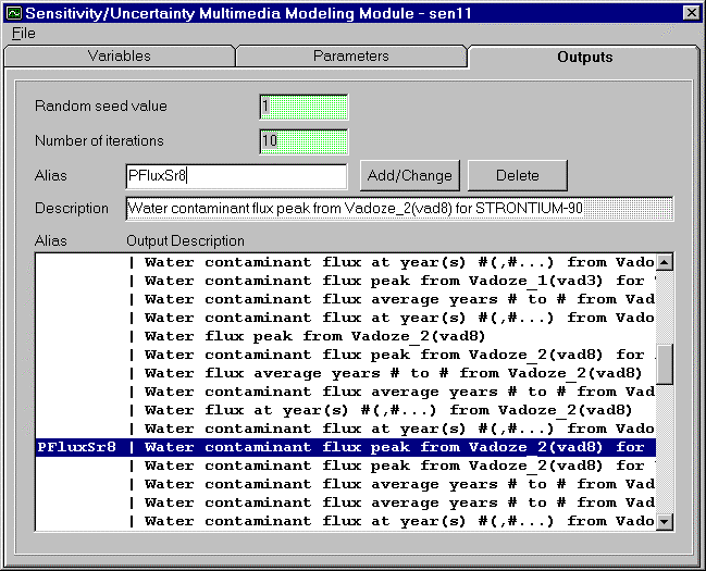
5.0 Selecting Output Variables of Interest
The Output tab enables users to specify the results to be preserved from simulation. The output list is provided for users with descriptions describing what results are and what module the output is from. This list of outputs is derived from all possible results produced from all media connected to the S/U icon. A description provides users with the output name and the module it is from (both the module name given by user and the FRAMES icon name are displayed). Figure 4.15 demonstrates a portion of the listing of outputs from two vadose zone modules and saturated zone module that have been connected to the S/U Module icon. A scroll bar is provided on the far right of the listing to enable users to move through the list when it is larger than the window length.
Adding Variable
The user is asked to provide a unique for each output of interest. To add, click on white entry box. Names should be one word (letters and numbers) and is limited to eight (8) digits, capitalization is preserved but is not used to distinguish between aliases, underscore symbol ( _ ) is not allowed. After typing, click Add button to enter into variable list. The output list will display to far left with a line ( | ) separating from description.
Changing Variable
An Add/Change button has been provided to allow a user to change existing . First select output to be changed. existing will appear in box. Enter new , and click Add/Change button. variable list will be updated with new .
Deleting Variable
A Delete button is provided to eliminate outputs from list for distributions. By removing from output list, output will no longer be preserved. This allows the user to reduce the listing to those currently of interest.
It is important to remember that only those outputs expected from modules connected to S/U module will be listed in this screen (i.e. user needs to be connected to aquifer icon if interested in waterborne concentration results from media). In addition to information, output screen also provides user with option to select seed value to be used in random sampling algorithm. Thereby allowing user to reproduce analysis if necessary. number of iterations (realizations) to be run is selected in on this tab also. number of iterations is number of sampling runs user would like to make. maximum number of iterations for a single simulation is 500.
6.0 Running the Sensitivity Uncertainty Module and SUM3
When all variable distributions, correlation, equations, and outputs have been selected and entered, the SUM3 model user interface can be closed.
Closing the SUM3 Module
To close the SUM3 module user interface, click the file menu and choose exit & save option. Choosing the Exit only option will not save any data changes made since the last time the user chose the exit & save option. This will return the user to the FRAMES interface.
Running the S/U Module
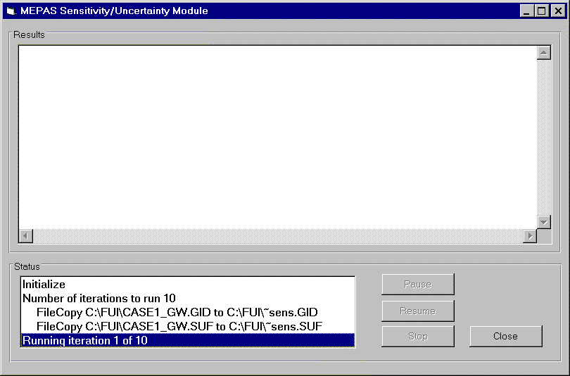
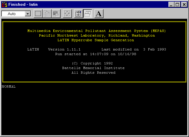
To run the S/U Module, shift-click the S/U Icon and select Run. While running the SUM3 model, a status screen will appear. Figure 6.1 illustrates the status screen. Figure 6.2 illustrates that the DOS screen appears to indicate the Latin Hypercube sampling tool has been activated and completed successfully. Close the DOS window to begin the calculation of sample iterations.
The FRAMES software is designed for deterministic models. Therefore, the SUM3 software product was designed to allow a statistical analysis using deterministic models. SUM3 will randomly sample input variables and preserve the associated output values in an external file available to the user for evaluation. The effect is calculating deterministic values with variable inputs producing a statistical distribution of results. A typical application of the uncertainty analysis is to indicate the relative conservatism of the deterministic result. Note that within the FRAMES software, the SUM3 model is located in the Sensitivity/Uncertainty Module.
6.1 Status Screen
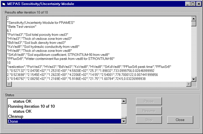
The status screen will identify the number of iterations (or realizations) that have been completed at the conclusion of each iteration. The statement "Iteration X of N" with a statement of OK or Error will appear. Figure 6.3 illustrates the status screen upon completion of the SUM3run. The status box will indicate completion of the simulation by displaying the word "DONE" in the lower left corner.
6.2 SUM3Sampling Technique
The FRAMES software is designed for deterministic models. Therefore, the SUM3 software product was designed to allow a statistical analysis using deterministic models. SUM3 randomly samples input variables following a Monte Carlo sampling method for correlated variables and a Latin Hypercube sampling method for uncorrelated variables. The listing of sampled input values is stored in the "runname".SUF (Sensitivity/Uncertainty File) file. Then SUM3 runs deterministic models once for each iteration, inserting the sampled value each time. After each deterministic run, the associated outputs of interest are preserved and also stored in "runname".SUF. A typical application of the uncertainty analysis is to indicate the relative conservatism of the deterministic result.
Monte Carlo Sampling Method
Latin Hypercube Sampling Method
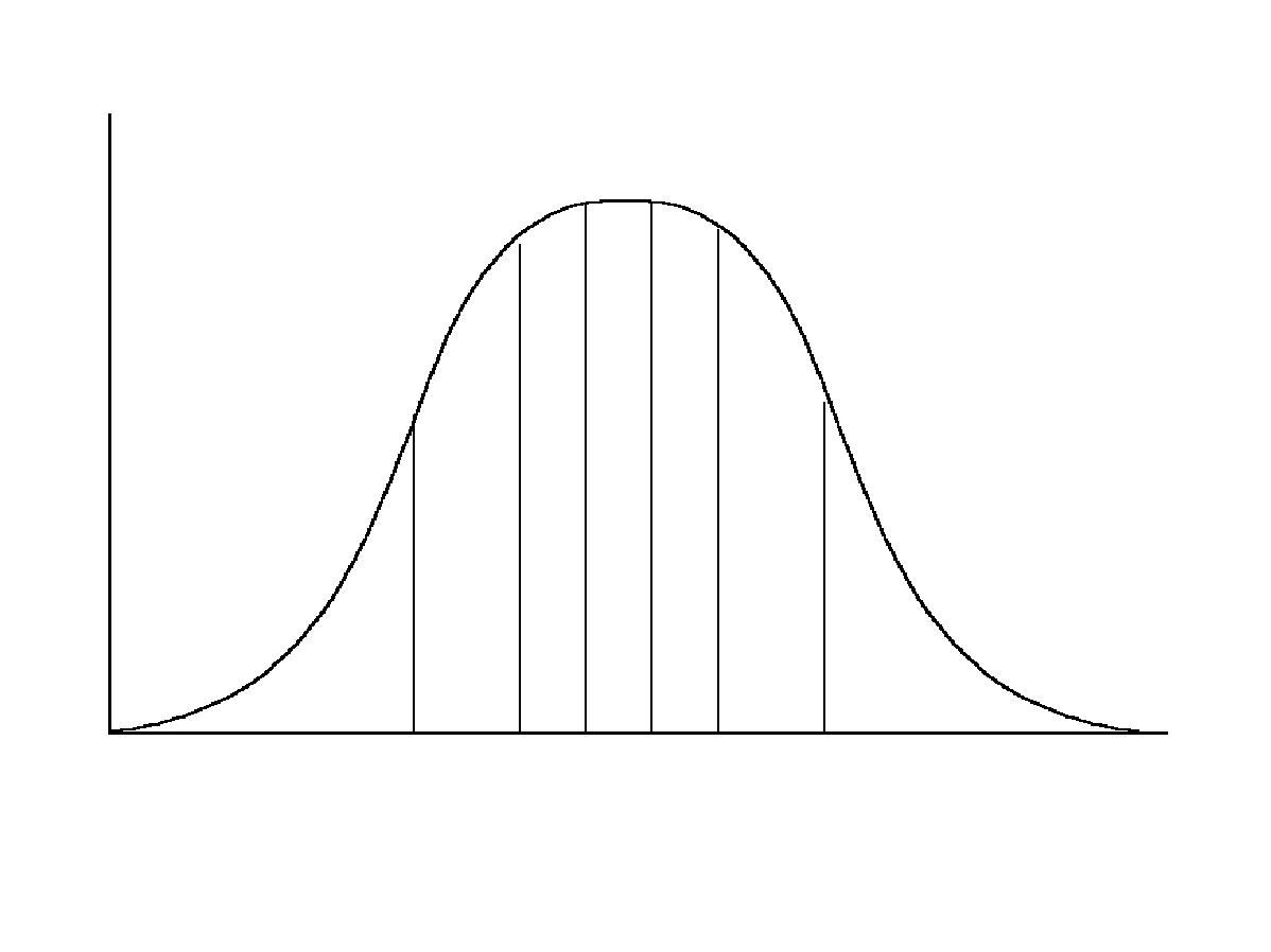
The Latin Hypercube method of sampling is a generalization of the Latin square experimental design to K dimensions, which correspond to the number of input variables selected of the model. Each input variable is assumed to be a random variable, which is governed by a probability density function (PDF). Stratification is accomplished by dividing the range of input variable into N intervals of equal (1/N) probability. Each equally probable interval is randomly sampled once for each variable. The output of sampling can be considered a NxK matrix, where columns represent variables and rows contain sample values for the appropriate interval. Values within a column are then randomly permuted, so a row represents a random vector of input variables. The environmental model is then run N times with the values of the input variables equal to therows of the matrix. Advantages of the Latin Hypercube sampling over unconstrained sampling methods are : 1) provides an efficient method for sampling the entire range of each variable in accordance with the assumed probability distribution. And an estimate of the PDF of the model output variables is an unbiased estimate of the true PDF. Latin Hypercube sampling methodology assumes that input variables are uncorrelated: however, this is not always the case in practice, and a simple Latin Hypercube sample may contain combinations of input variables that are physically unreasonable. Iman and Conover (1982) developed a method to induce desired the dependence among variables in a Latin Hypercube sampling using a rank correlation matrix. The method is very effective when a rank correlation among all pairs of variables can be obtained (Doctor et al. 1988). Figure 6.4 illustrates this concept in which a parameter´s probability distribution is divided into intervals of equal probability. Compared with the conventional Monte Carlo sampling, Latin Hypercube sampling is more precise because the entire range of the distribution is sampled in a more even and consistent manner.
7.0 Interpreting Results
Results from a sensitivity/uncertainty analysis can be used to derive the confidence limits and intervals to provide a quantitative statement about the effect of varying a parameter on the model prediction. The sampled variables, along with their associated outputs of interest, are stored in a file. This data is stored in a comma-separated format and stored in a file named "runname".SUF, where "runname" is the filename given to the FRAMES case analysis. Figure 7.1 illustrates an example SUF file with notations identifying key information.
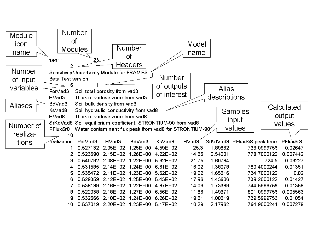
The file format for the SUF file is also consistent with the necessary information to complete an r-squared analysis in a more sophisticated statistical tool such as SAS.
Example file
SUM3´s charting feature enables users to view results. Cumulative Distribution Function (CDF) curves are options for viewing the results.
8.0 Example Illustrating Application of Sensitivity Uncertainty Module
Chapters 1 through 6 present a user´s guide to the operating of the sensitivity uncertainty module. Although a user might find this guidance helpful, a real-world application of software within the context of a source, fate and transport, and exposure and risk/hazard assessment also tends to be informative. This chapter presents an application of the sensitivity uncertainty module as a component of a real-world hazardous waste site assessment exercise.
8.1 Introduction
The objective of the assessment is to determine if the Waste Management Unit (WMU) requires a more in-depth analysis, including a more rigorous monitoring plan. A preliminary probabilistic assessment is performed, using semi-analytical modeling techniques, to help quantify a safety envelope. Such risks will be no larger than those presented. Based on these results, a qualitative decision can be made as to follow-on action items, which will not be discussed within this chapter, as only the assessment process is presented. Because this assessment represents an illustrative example, the actual site has not been identified.
8.2 Background
In 1985, a 650-gal Underground Storage Tank (UST) was installed to a depth not exceeding four meters. The tank was used to store used diesel #1 and #2 fuel. The soil surrounding the tank resembled silty clay, which sits on a fractured shale. The water table is perched with depths of one-third to one meter. Hydrogeologically, the area is a mound where water tends to flow radially in all directions, although the tank is located at one end of this mound with the water primarily moving in one direction. In 1994, the tank was physically removed from service. During the excavation process, it became evident that the tank had leaked, thereby becoming a Leaking Underground Storage Tank (LUST). Although site data are scarce, several samples were collected to initially quantify contamination. The constituents of interest were Benzene, Toluene, Ethylbenzene, and Xylene (BTEX), naphthalene, and trichloroethylene (TCE).
The Framework for Risk Analysis in Multimedia Environmental Systems (FRAMES) was used as a platform for performing a preliminary probabilistic assessment, using semi-analytical modeling techniques, to help quantify a safety envelope. Such risks will be no larger than those presented (Whelan et al. 1997). The computer model used to perform all the modeling runs within the FRAMES platform was the Multimedia Environmental Pollutant Assessment System (MEPAS©) (Buck et al. 1995; Whelan et al. 1992). MEPAS© is a physics-based environmental analysis code that integrates source-term, transport, and exposure models for endpoints such as concentration, dose, or risk. MEPAS© was developed by the Pacific Northwest National Laboratory for use in site-specific assessments such as this.
8.3 Predictive and Comparative Assessments
The multimedia site-specific risk assessments are traditionally modeled using one of two modes--predictive or comparative. In a predictive assessment, models are calibrated to the monitored data to identify the representative hydrodynamic and hydrogeologic values of parameters within the acceptable ranges. The intent of calibration is to ensure that environmentally monitored concentrations are recreated by the model in magnitude, location, and time. This is best done with multiple sets of monitored data, which consider multiple and interrelated chemicals at multiple locations occurring at multiple times. Once calibrated, the information can not only be used to assess the calibrated chemicals, but it can also be used to assess other chemicals that may be present at site but whose conditions do not allow for calibration.
A comparative assessment recreates conditions as they might be without calibrating to monitored data. Under this situation, an analyst investigates ramifications of differing "what-if" scenarios, as defined by the analyst. The scenarios do not necessarily have to be realistic. For example, if the analyst wants to quickly determine under a bounding worst-case scenario, if risks are below 10-6, the analyst may assume that a receptor is directly exposed to waste. Although this scenario may be impossible, the analysis does not need to proceed further if the risks calculate to less than 10-6, as the criterion for additional analyses (i.e., risk greater than 10-6) is never exceeded. In this case, the analyst does not require the "correct" number (i.e., risk) to make the "right" decision. This type of analysis attempts to bound problems within a conservative assessment. The intent of the analysis is to identify the region that is unlikely or impossible to occur.
At this site, both a predictive and comparative analysis are used to identify the ramifications of the 650-gal waste diesel-oil leaking underground storage tank. The constituents xylene, toluene, and ethylbenzene are employed in a predictive assessment to not only recreate their concentrations in environment at different locations and times, but also to estimate a representative hydrodynamic and hydrogeologic situation (within acceptable bounds), which can be employed to analyze the potential impacts of other constituents at the site in a comparative mode. Naphthalene, trichloroethylene, and benzene, which represent constituents that have exceeded acceptable thresholds, represent chemicals that are assessed in a comparative mode to determine if additional analyses are required.
8.4 Predictive Assessment
The objective of the predictive assessment is to ascertain the representative hydrogeologic and hydrodynamic properties that reflect the characteristics of chemical migration and fate at the site. The values of specified parameters are determined in the calibration process to match the monitored data. In this assessment, ethylbenzene, toluene, and xylene were simultaneously calibrated to the monitored concentrations at two different well locations. Such calibrations maintained the same consistent set of hydrogeologic and hydrodynamic properties. The following sections: 1) describe the calibration process, 2) present calibration parameters and results, and 3) discuss probabilistic human-health risk results to ascertain the possible adverse human-health hazards.
8.4.1 Calibration Process
As in any groundwater modeling exercise, the spacial and temporal descriptions of concentrations at any location are functions of a constituent´s release history and the physical and hydrogeologic characterization of the aquifer. Because every groundwater model, no matter how complex, represents a simplification of the real world, the intent of a calibration exercise is to anchor the modeling to reality (i.e., to monitored environmental data). As such, values for the release history and the hydrogeologic parameters are varied (within reason) and defined to recreate monitored environmental data. The greater number of constraints on the calibration exercise, the more accurate the description. For example, calibrating to multiple data points [e.g., multiple chemicals (with different physical and chemical characteristics)] to multiple locations using the same flow information (e.g., pore water velocity, porosity, soil type, etc.) is much more difficult and provides more accurate results than calibrating to one data point (e.g., one chemical at one time and location).
This site contains soil that has been contaminated with petroleum hydrocarbons, possibly attributable to the 650-gal LUST, which contained used diesel fuel. Diesel fuel (i.e., diesel fuel #1 and #2) is typically composed of 0.004, 0.014, 0.03, 0.20, and 0.20 percent by weight of benzene, toluene, ethylbenzene, xylene, and naphthalene, respectively (USAF 1993). The possible route of the subsurface constituent migration includes leaching of contamination through a short silty-clay vadose zone and a migration through a one-third to one meter thick perched silty-clay aquifer, which sits on a fractured shale. Constituent transport through the fractured rock was not simulated. Although the perched aquifer sits above a fractured shale, concern is associated with the possible exposure to contamination migrating from the source to downgradient locations through the silty-clay. MW-2 and MW-4 represented downgradient locations associated with the calibration exercise. There are three similar yet different approaches for modeling the constituent migration from the source to monitoring wells. Each becomes conceptually more simple, and the choice of most the appropriate conceptual site model is a function of available data:
- The first conceptual site model consists of a source of contamination migrating through a vadose zone to a saturated zone, then being transported via groundwater flow through the perched aquifer to monitoring wells MW-2 and MW-4, where the modeled concentrations would be compared and calibrated to the monitored data.
- If data are lacking to adequately describe the phenomenological mechanisms governing the release and transport of constituents through the vadose zone, then the second scenario would assume a time-varying release directly to the saturated zone, not describing transport through but accounting for the transport from the vadose zone. A horizontal source plane would be assumed to be at the water table, providing a contaminated source to the saturated zone where it would be transported via groundwater flow through the perched aquifer to the monitoring wells MW-2 and MW-4, where modeled concentrations would be calibrated to the monitored data.
- If the release mechanisms from the vadose zone to the saturated zone linked with vertical mixing mechanisms in the saturated zone are not well understood, the third conceptual site model consists of a constituent flux crossing a vertical plane in the aquifer, extending from the water table to the aquifer bottom. Contamination in the saturated zone would then be transported downgradient via the groundwater flow through the perched aquifer and to monitoring wells MW-2 and MW-4, where the modeled concentrations would be calibrated to the monitored data.
Calibration exercises associated with the first two conceptual site models were implemented, but, due to lack of data and a full understanding of the current phenomenological mechanisms governing constituent migration through and release from the vadose zone, the third conceptual site model (i.e., constituent flux passing through a vertical plane in the aquifer) was eventually employed. The third conceptual site model was used to ensure that the calibration parameters varied within the acceptable bounds and made physical sense. Using this source release mechanism, it was possible to calibrate three constituents, using consistent hydrogeologic and hydrodynamic conditions, to the constituent groundwater concentrations at monitoring wells MW-2 and MW-4.
8.4.2 Calibration Parameters and Results
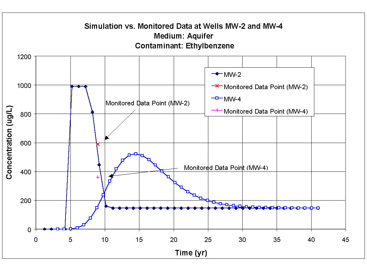
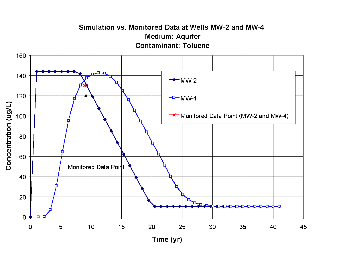
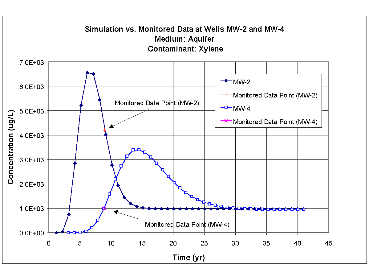
Xylene, toluene, and ethylbenzene were used in the calibration exercise to determine values for the hydrogeologic parameters because the monitored data were available. Measured concentrations were available for these three constituents at MW-2 and MW-4, respectively, and they appeared to be indicative of plume migration in the aquifer. Table 8.1 presents the monitored groundwater concentrations at monitoring wells MW-2 and MW-4 for ethylbenzene, toluene, and xylene for 1994, which is 9 years after the 650-gal tank was installed.
Table 8.1. 1994 Monitored Ground Water Concentrations for Ethylbenzene, Toluene, and Xylene at MW-2 and MW-4| Constituent | Monitored Concentration at MW-2 (mg/L) | Monitored Concentration at MW-4 (mg/L) |
|---|---|---|
| Ethylbenzene | 590 | 360 |
| Toluene | 130 | 130 |
| Xylene | 4,200 | 1,000 |
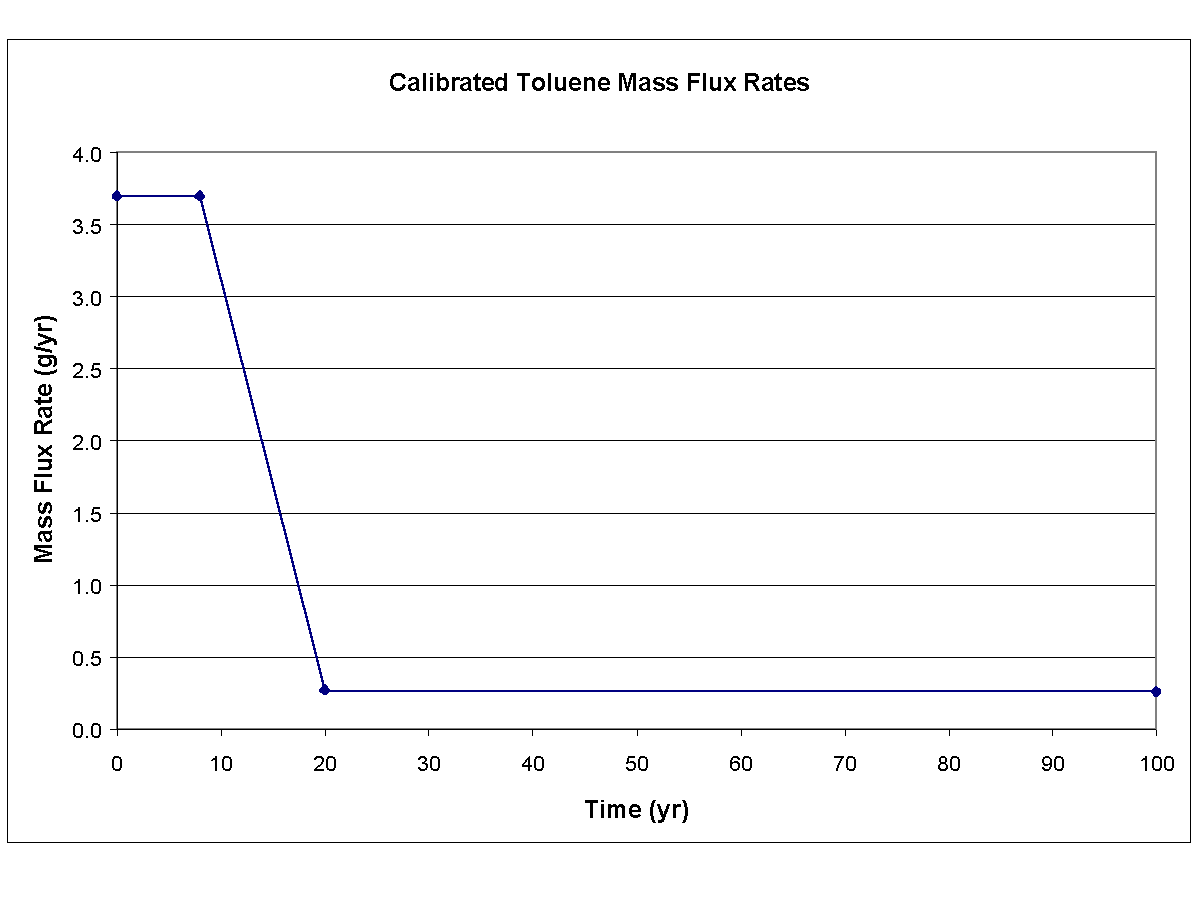
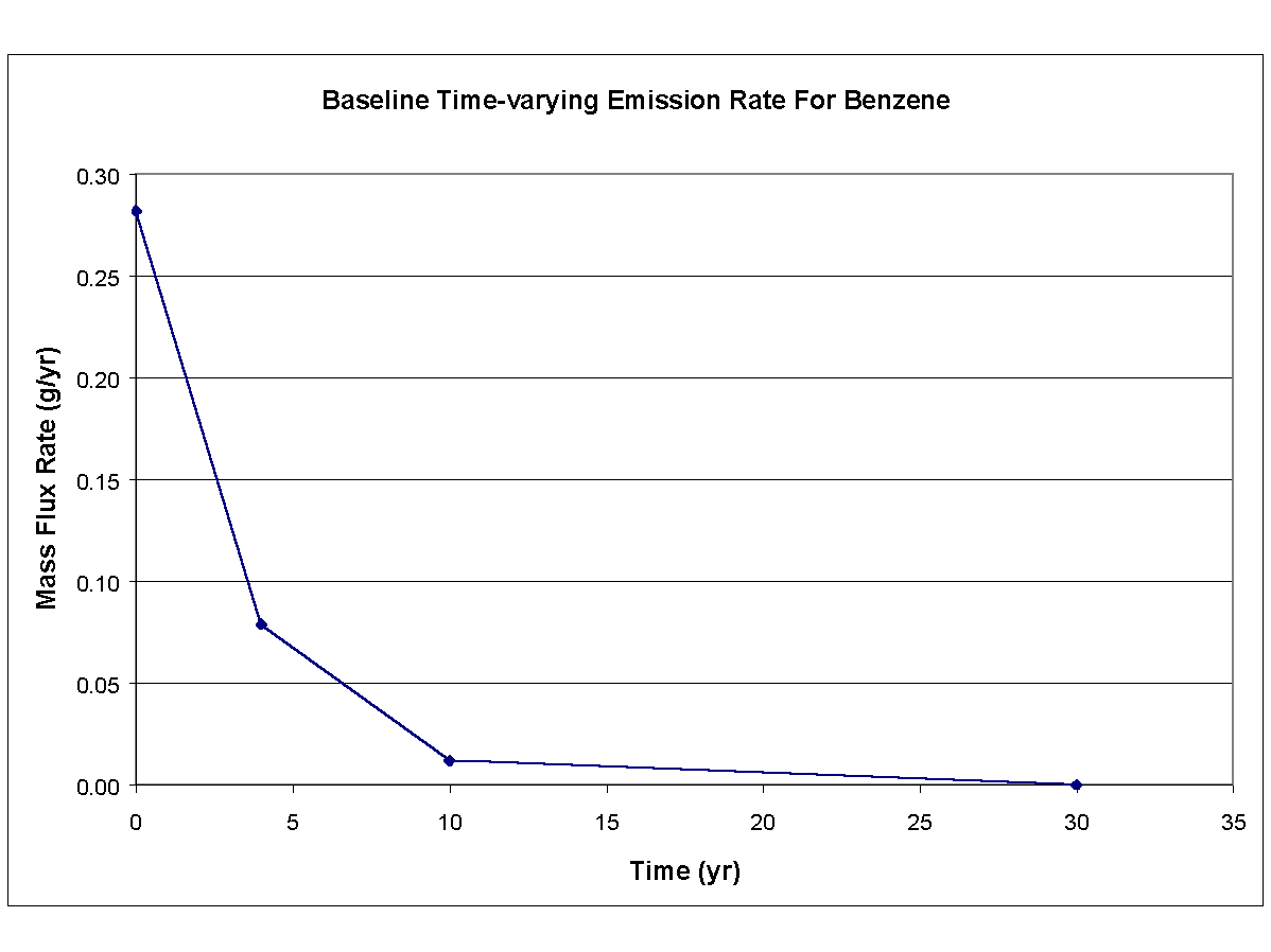
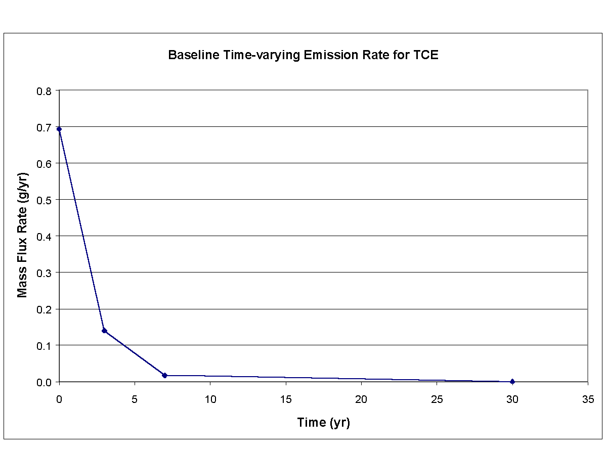
The hydrogeologic and hydrodynamic properties of the aquifer were gathered from reports and from personal inspection of the site. Because these three constituents were released into the same perched aquifer, values for the hydrogeologic and hydrodynamic parameters had to be consistent. Table 8.2 presents the values for the hydrogeologic and hydrodynamic parameters used in calibration and simulation exercises. In addition to the parameters identified in Table 8.2, the time-varying mass flux rates through the vertical plane in the aquifer for ethylbenzene, toluene, and xylene also represented calibration parameters. The calibrated time-varying mass flux rates for ethylbenzene, toluene, and xylene are presented in Figures 8.1, and 8.2 respectively.
Table 8.2. Calibrated Hydrogeologic and Hydrodynamic Parameters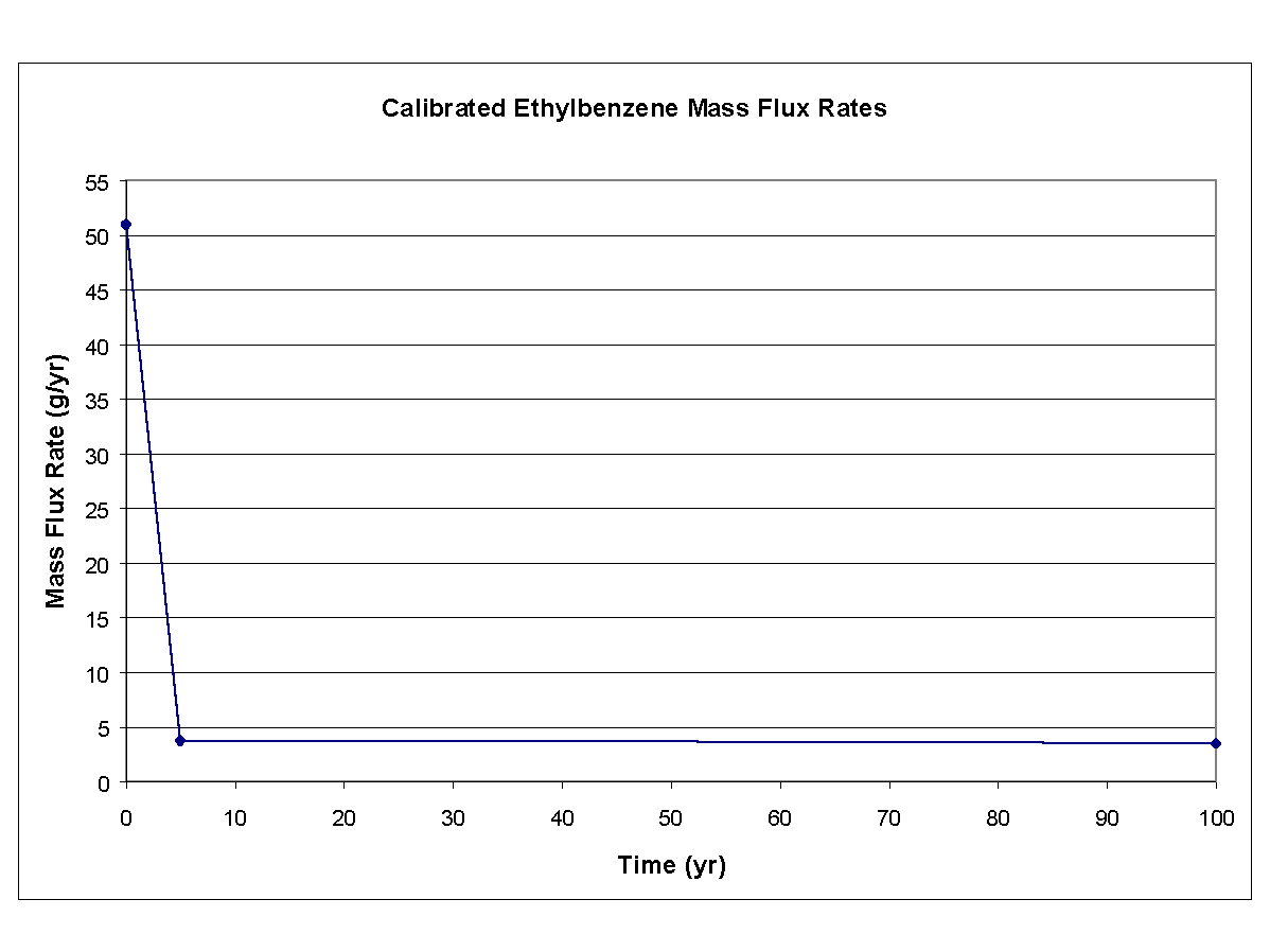
| Parameter | Value | Units | Reference |
|---|---|---|---|
| Total Porosity | 36.0 | % | Calculated |
| Effective Porosity | 36.0 | % | Calibrated |
| Darcy Velocity | 0.72 | cm/d | Calibrated |
| Thickness of Aquifer | 0.61 | m | Site Data |
| Dry Bulk Density | 1.7 | g/cm3 | Assumed |
| Longitudinal Distance to MW-2 | 3.5 | m | Site Data |
| Perpendicular Distance From Plume Center Line to MW-2 | 0.0 | m | Site Data |
| Vertical Distance Below Water Table at MW-2 | 0.0 | m | Assumed |
| Longitudinal Dispersivity for MW-2 | 0.175 | m | Calibrated |
| Transverse Dispersivity for MW-2 | 0.0289 | m | Calibrated |
| Vertical Dispersivity for MW-2 | 0.0004 | m | Calibrated |
| Longitudinal Distance to MW-4 | 8.9 | m | Site Data |
| Perpendicular Distance From Plume Center Line to MW-4 | 0.0 | m | Site Data |
| Vertical Distance Below Water Table at MW-4 | 0.0 | m | Assumed |
| Longitudinal Dispersivity for MW-4 | 0.445 | m | Calibrated |
| Transverse Dispersivity for MW-4 | 0.734 | m | Calibrated |
| Vertical Dispersivity for MW-4 | 0.001 | m | Calibrated |
| Ethylbenzene Kd | 2.0 | mL/g | Calibrated |
| Toluene Kd | 0.7 | mL/g | Calibrated |
| Xylene Kd | 2.0 | mL/g | Calibrated |
The results of calibration process are presented in Figures 8.4, 8.5, and 8.6, which present the time-varying simulated results and the monitored data points for ethylbenzene, toluene, and xylene, respectively, at monitoring wells MW-2 and MW-4. Time zero in each plot refers to 1985, and the monitored data points correspond to nine years after the 1985 installation of the 650-gal tank (i.e., 1994). It was assumed that the tank leak started in 1985 because no information was available that described the leak.
8.4.3 Probabilistic Human-Health Risk Assessment for Ethylbenzene, Toluene, and Xylene
Following the calibration exercise, a probabilistic human-health risk assessment was performed to ascertain if ethylbenzene, toluene, and xylene contamination posed a significant human-health risk, as shown by the risk assessment approach in the U.S. Environmental Protection Agency (EPA) Risk Assessment Guidelines for Superfund (RAGS) (EPA 1989). Because there are no receptor locations (e.g., drinking-water wells) in the near vicinity of the waste site, several hypothetical, yet conservative, receptor locations and scenarios were identified. Analyses were performed at 10-, 50-, and 100-m distances from the center of the source. Other conservative assumptions were also implemented. For example, losses due to degradation or volatilization were not considered. Also, the aquifer was assumed to be present throughout the length of the modeling period. This may or may not reflect reality at this site. Several of the monitoring wells were found to be nearly dry during the sampling exercises. This suggests that the perched aquifer was not always present. Table 8.3 presents parameters that describe the exposure scenario used in the risk assessment. Included in Table 8.3 are cancer potency factors (i.e., slope factors) and reference doses used in calculations for risk (i.e., cancer incidence for carcinogens) and hazard quotient (for non-carcinogens), respectively. Under this scenario, a 70-kg adult individual is assumed to obtain all drinking water from this aquifer at a rate of 2 L/d over a lifetime exposure period of 30 yr.
Table 8.3. Exposure Parameters| Parameter | Value | Units |
|---|---|---|
| Exposure Pathway | Drinking Water | none |
| Exposure Duration | 30 | yr |
| Is Water Treated? | No | none |
| Body Weight of Individual | 70.0 | kg |
| Drinking Water Ingestion Rate | 2.0 | L/d |
| Ethylbenzene Reference Dose a | 1.0E-1 | mg/(kg-d) |
| Toluene Reference Dose b | 2.0E-1 | mg/(kg-d) |
| Xylene Reference Dose c | 2.0 | mg/(kg-d) |
| Benzene Slope Factor d | 2.9E-2 | (kg-d)/mg |
| Naphthalene Reference Dose e | 4.0E-2 | mg/(kg-d) |
| TCE Slope Factor f | 1.1E-2 | (kg-d)/mg |
|
a EPA Integrated Risk Information System (IRIS), 06/01/91, http://www.epa.gov/IRIS/subst/0051.htm#I.A. b EPA IRIS, 04/01/94, http://www.epa.gov/IRIS/subst/0118.htm#I.A. c EPA IRIS, 09/30/87, http://www.epa.gov/IRIS/subst/0270.htm#I.A. d EPA IRIS, 04/01/97, http://www.epa.gov/IRIS/subst/0276.htm e EPA Health Effects Assessment Summary Tables (HEAST), 1992, Office of Solid Waste and Emergency Response, NTIS/PB92-921199 f EPA, 1984, Health Effects Assessment for TCE Final Draft, Environmental Criteria and Assessment Office, Cincinnati, OH, ECAO-CIN-H0O9 |
||
To account for the uncertainty associated with parameters employed in the modeling exercise, a Monte Carlo analysis was implemented, using the Latin Hypercube Sampling technique. The advantage of Latin Hypercube sampling over unconstrained sampling is that the Latin Hypercube sampling provides an efficient method for sampling the entire range of each variable in accordance with the assumed probability distribution (Doctor et al., 1990). Five hundred realizations were implemented for each chemical at each of the three locations to present the probability of exceedence versus risk (i.e., hazard quotient) versus distance. In each realization, the values for stochastic parameters were randomly chosen within reasonable ranges. Tables 8.4 and 8.5 present each stochastic parameter and its corresponding distribution, maximum, mean, minimum, and standard deviation. In effort to account for as much uncertainty as possible, a conservative estimate of the standard deviation was used and defined as the range (i.e., range = maximum-minimum) divided by three. One-third is approximately twice a typical definition of standard deviation when it is unknown, which is typically defined as the range divided by six. For example, if the hydrogeologic parameters in Meyer et al. (1997) for silty clay are summarized for a normal distribution, the standard deviation statistically calculates to be the range divided by 5.8± 0.4, where 0.4 represents a 95% confidence interval of the mean of the observations, using a Student-t distribution for a small sample (APHA 1986).
Table 8.4. Stochastic Saturated Zone Parameters| Parameter | Distribution | Max. Value | Mean Value | Min. Value | Std. Dev. | Units |
|---|---|---|---|---|---|---|
| Source Width | Uniform | 20.0 | none | 12.0 | none | m |
| Source height | Uniform | 1.0 | none | 0.31 | none | m |
| Water Flux | Uniform | 105.0 | none | 2.0 | none | m3/yr |
| Bulk Density | Normal | 1.9 | 1.7 | 1.7 | 0.067 | g/cm3 |
| Longitudinal Dispersivity (10 m) | Normal | 100.0 | 50.0 | 25.0 | 25.0 | cm |
| Longitudinal Dispersivity (50 m) | Normal | 500.0 | 250.0 | 125.0 | 125.0 | cm |
| Longitudinal Dispersivity (100 m) | Normal | 1000.0 | 500.0 | 250.0 | 250.0 | cm |
| Ethylbenzene Kd | Normal | 5.0 | 2.0 | 1.0 | 1.3 | mL/g |
| Toluene Kd | Normal | 4.0 | 0.7 | 0.1 | 1.3 | mLg |
| Xylene Kd | Normal | 5.0 | 2.0 | 1.0 | 1.3 | mL/g |
Table 8.5. Stochastic Constituent Flux Data in Predictive Assessment
| Parameter | Distribution | Max. Value | Mean Value | Min. Value | Std. Dev. | Units |
|---|---|---|---|---|---|---|
| Ethylbenzene Flux at t = 0 yr | Normal | 51.0 | 51.0 | 25.6 | 8.467 | g/yr |
| Ethylbenzene Flux at t = 5 yr | Normal | 7.5 | 3.75 | 1.875 | 1.875 | g/yr |
| Toluene Flux at t = 0 yr | Normal | 7.4 | 3.7 | 1.85 | 1.85 | g/yr |
| Toluene Flux at t = 20 yr | Normal | 0.54 | 0.27 | 0.135 | 0.135 | g/yr |
| Toluene Flux at t = 15525 yr | Normal | 0.066 | 0.017 | 0.033 | 0.017 | g/yr |
| Xylene Flux at t = 0 yr | Normal | 340.0 | 340.0 | 170.0 | 56.7 | g/yr |
| Xylene Flux at t = 5 yr | Normal | 50.0 | 25.0 | 12.5 | 12.5 | g/yr |
Table 8.4 presents the stochastic parameters not associated with release information, while Table 8.5 presents stochastic information associated with time-varying mass flux rates for each of three chemicals. The mean values reported in Table 8.5 correspond to curves that are presented in Figures 8.1, and 8.2. Ranges for each of the parameters were defined so as not to violate basic hydrogeologic and hydrodynamic principles. For example, 1) concentrations cannot be greater than the solubility limit, 2) effective porosity cannot be greater than the total porosity, and 3) maximum constituent velocity cannot not be less than the actual constituent velocity that was observed at the site. Because many of the parameters are interrelated, their ranges must also reflect these interrelationships during the random sampling associated with the Monte Carlo assessment to maintain credibility and accuracy. For example, source constituent emission rates that occur later in time cannot have higher magnitudes assigned to them than the emissions rates that occur earlier in time.
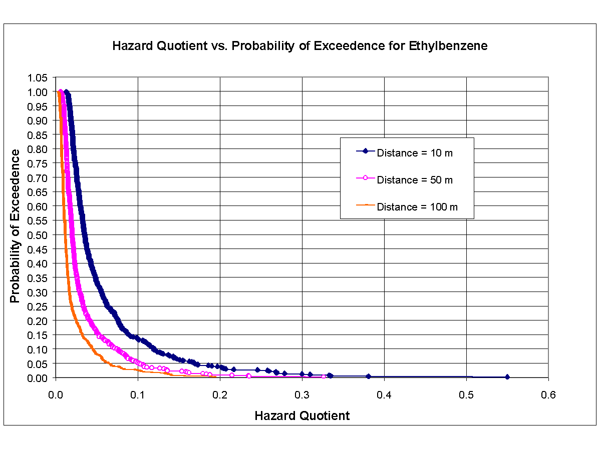
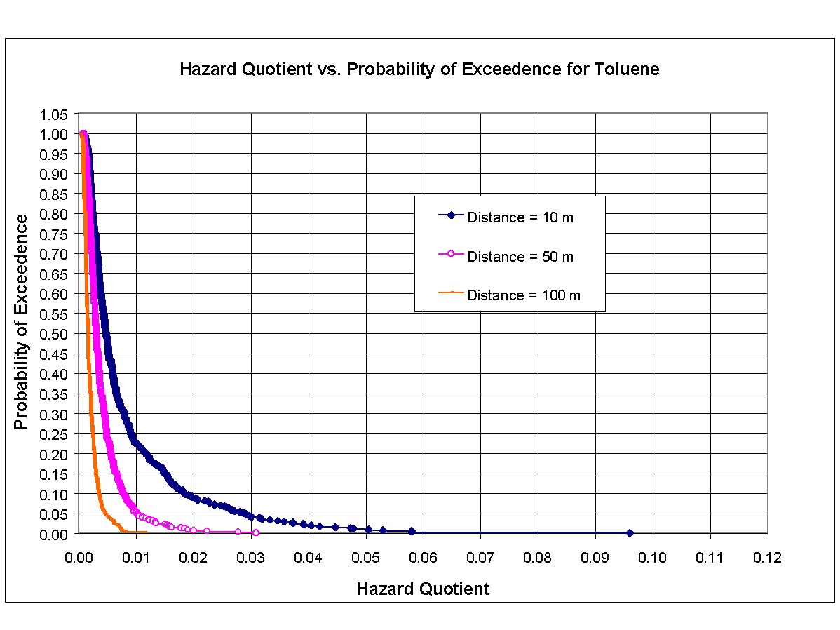
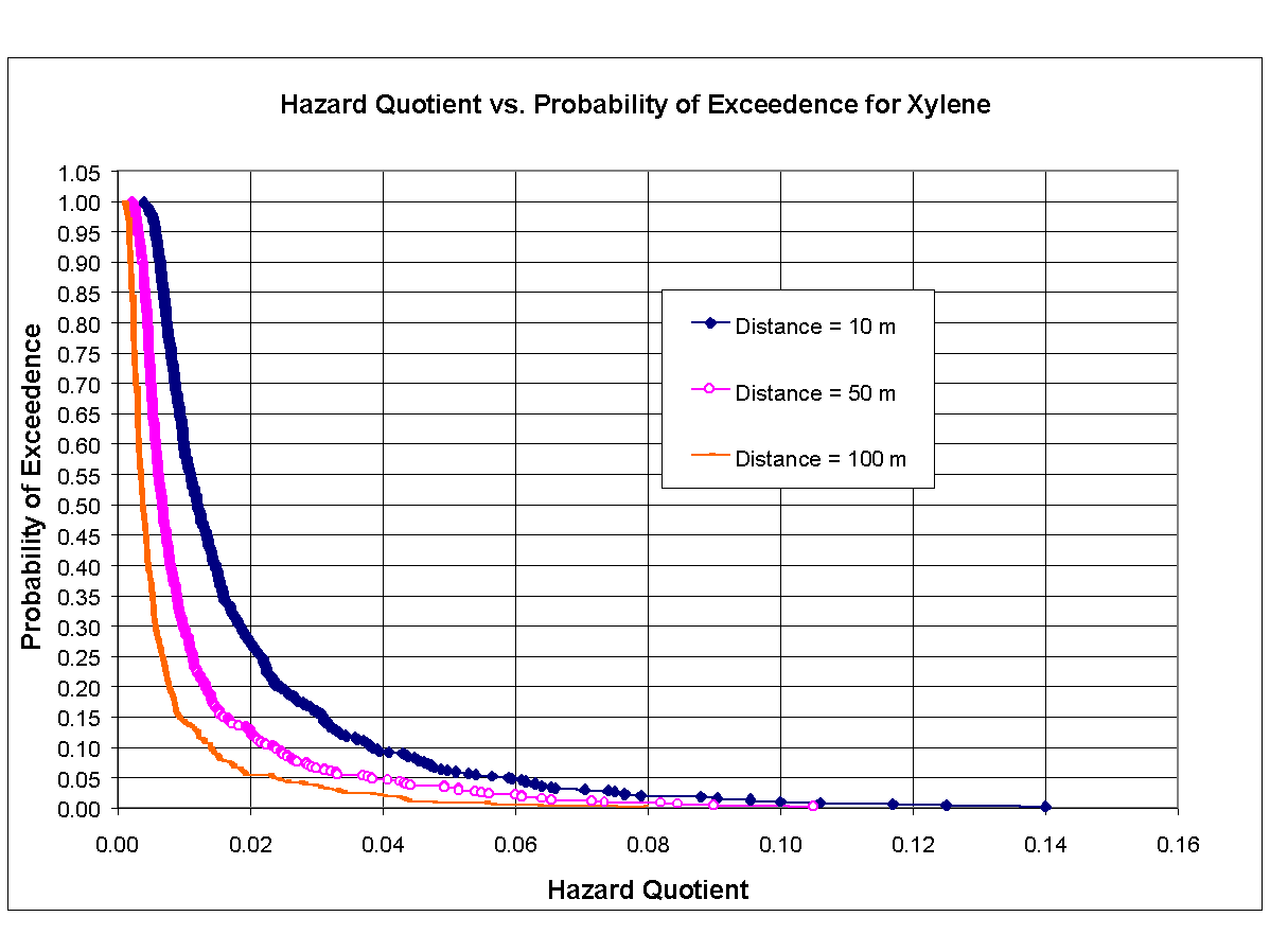
Figures 8.7, 8.8, and 8.9 are cumulative distribution function (CDF) curves developed from results of Monte Carlo analysis, corresponding to noncarcinogenic chemicals ethylbenzene, toluene, and xylene, respectively. CDF curves in each figure correspond to distances from center of source of 10, 50, and 100 m and plot probability of exceedence versus hazard quotient. As can be seen in these figures, probability of exceeding unity is nearly zero for all three constituents at all three distances.
8.5 Comparative Assessment
Although a risk assessment was implemented on ethylbenzene, toluene, and xylene, no monitored constituent levels attributed to these chemicals exceeded the acceptable regulatory limits. The assessment of these chemicals was useful, though, as they provided a basis for calibrating and anchoring the computer model to monitored data. In addition, their analysis allowed for the determination of hydrodynamic and hydrogeologic parameters that can be used in the assessment of other less-documented chemicals attributed to the site--chemicals that have constituent levels with at least one measurement exceeding a regulatory limit.
Benzene, naphthalene, and trichloroethylene (TCE) have at least one recorded concentration that exceeds the regulatory limit for groundwater. The regulatory limits for benzene, naphthalene, and TCE are 5, 20, and 5 m g/L, respectively, and the maximum concentration recorded at least once are 11, 41, and 27 m g/L. Unlike ethylbenzene, toluene, and xylene, whose contamination tended to be centered near the 650-gal LUST and tended to follow groundwater-flow contours, the maximum concentrations for benzene, naphthalene, and TCE tended to be centered near a storm-water drain near monitoring well MW-5, which was located 13 m from the tank perpendicular to the groundwater flow direction. As with ethylbenzene, toluene, and xylene, the source-release information was not available for these three constituents. Additionally, monitored data available for these three constituents were not adequate to estimate a source-release pattern with a calibration exercise. A comparative assessment, therefore, was employed as a means of bounding possible source releases, as well as assessing various scenarios to examine if constituents realistically pose human-health hazards.
8.5.1 Comparative Assessment Scenarios
For source terms that do not contain free product (i.e., concentration exceeding solubility limit), the rate of contamination that is released from a source is typically auto-correlated to the amount of mass remaining at the source (Codell et al. 1982). In other words, as the source is depleted over time (both in mass and size), the rate of the release of contamination also decreases with time. In effect, this release pattern accounts for 1) initial higher level of release, as might be expected when contamination initially occurs, and 2) a lower level of release, as might be expected when residual contamination "bleeds" from the source. The assumption of auto-correlation is utilized in this comparative assessment.
Three different assessment scenarios, using auto-correlation assumption, were implemented to help frame a conservative analysis, placing benzene, TCE, and naphthalene contamination within a human-health risk assessment context. Each scenario is described as follows:
- One bounding auto-correlation scenario is to assume that the release duration is so short that it can be approximated by an instantaneous release.
- A second bounding auto-correlation scenario is to assume that the release pattern can be approximated as a constant release. This second scenario can be extremely conservative, as a constant release pattern generally implies 1) the presence of free product, as the level of contamination would remain constant at the source or 2) the mass at the source is significantly larger than the rate of release from the source.
- In a third scenario, maximum monitored concentration is assumed as the initial source concentration, and a probabilistic analysis is implemented.
Scenarios 1 and 2 compared how the simulated maximum concentration must exist in the groundwater at the source, which corresponded to a risk of 10-6 or HQ of unity at the receptor location, to the maximum recorded concentration. In other words, if the simulated maximum concentration at the source is higher than the recorded maximum concentration at the source, then the risk or HQ at the receptor location cannot equal or exceed 10-6 or 1.0, respectively.
Scenarios 1 and 2 were implemented as a filtering or screening step prior to the implementing of Scenario 3. If the simulated maximum concentration was significantly higher than the recorded maximum concentration, then the constituent would be removed from further consideration, as the risk or HQ would be below 10-6 or unity, respectively, and the implementation of Scenario 3 would not be necessary.
8.5.2 Deterministic Assessment (Scenarios 1 and 2)
Scenarios 1 and 2 employed hydrodynamic, hydrogeologic, exposure, receptor, and health-impact assumptions developed under the predictive assessment exercise, as suggested in Tables 8.1, 8.2, and 8.3, except for the constituent specific parameters and dispersivity, where dispersivity varies with distance. Distribution coefficients (i.e., Kds) for benzene, naphthalene, and TCE were defined as 2.0, 1.7, and 2.1 ml/g, respectively. The mass flux releases were determined as part of the bounding exercise. Included in Table 8.3 are cancer potency factors (i.e., slope factors) and reference doses used in calculations for risk (i.e., cancer incidence for carcinogens) and a hazard quotient (for non-carcinogens), respectively. In addition, a 70-kg adult individual is assumed to obtain all drinking water from this aquifer at a rate of 2 L/d over a lifetime exposure period of 30 yr.
For benzene, naphthalene, and TCE, it was assumed that allowable threshold limits for human health at the site were a risk of 10-6 for carcinogenic constituents (i.e., benzene and TCE) and a HQ of 1.0 for non-carcinogens (i.e., naphthalene). These limits were used to establish bounding conditions for the constituent releases and source-term concentrations. Modeling runs were performed to determine the release characteristics that would be required to reach a HQ of 1.0 or a risk of 10-6 through drinking-water ingestion. Because there are no actual receptors located in the vicinity of the site, a hypothetical receptor was in place at the border of the facility, which was estimated to be 100 m from the source. This represented the closest possible distance a drinking-water well might be installed, regardless of whether the well would be productive. The results of the bounding exercise are presented by the constituent in the following sections.
Naphthalene
- Scenario 1 (instantaneous release) -- To reach a HQ of unity at a distance of 100 m, nearly 7.4 kg would have to be instantaneously released at a concentration of over 69 mg/L, using a Darcy velocity of 0.72 cm/d. A constituent concentration this high is not only implausible but also impossible because the solubility limit of naphthalene is only 34 mg/L.
- Scenario 2 (constant release) -- To reach a HQ of unity at a distance of 100 m, nearly 22 kg would have to be released over 280 yr at a constant concentration of nearly 3 mg/L, using a Darcy velocity of 0.72 cm/d. A water concentration this high is over 70 times larger than highest monitored concentration of 0.041 mg/L.
Based on these results, naphthalene was eliminated from further analysis (i.e., Scenario 3 was not implemented), as these results clearly indicate that naphthalene does not pose a significant health hazard at a distance of at least 100 m.
- Scenario 1 (instantaneous release)--To reach a risk of 10-6 at a distance of 100 m, the source would have to have a concentration of nearly 140 m g/L, using a Darcy velocity of 0.72 cm/d. A water concentration this high is over 10 times larger than the highest monitored concentration of 11 m g/L.
- Scenario 2 (constant release)--To reach a risk of 10-6 at a distance of 100 m, over 44 g would have to be released over 280 yr at a constant concentration of over 6 m g/L, using a Darcy velocity of 0.72 cm/d. Although the initial mass of 44 g and the duration of the release of 280 yr at a constant concentration are high, the simulated constant concentration of 6 m g/L is less than the highest monitored concentration of 11 m g/L.
To err on the side of conservatism, benzene was included in a probabilistic assessment because the simulated concentration of 6 m g/L (assumed constant over 280 yr) was less than the maximum monitored concentration of 11 m g/L.
- Scenario 1 (instantaneous release)--To reach a risk of 10-6 at a distance of 100 m, the source would have to have a concentration of over 360 m g/L, using a Darcy velocity of 0.72 cm/d. A constituent concentration this high is over 13 times larger than the highest monitored concentration of 27 m g/L.
- Scenario 2 (constant release)--To reach a risk of 10-6 at a distance of 100 m, over 140 g would have to be released over 340 yr at a constant concentration of over 16 m g/L, using a Darcy velocity of 0.72 cm/d. Although the initial mass of 144 g and the duration of a release of 340 yr at a constant concentration are high, the simulated constant concentration of 16 m g/L is less than the highest monitored concentration of 27 m g/L.
To err on the side of conservatism, TCE was included in a probabilistic assessment because the simulated concentration of 16 m g/L (assumed constant over 340 yr) was less than the maximum monitored concentration of 27 m g/L.
8.5.3 Probabilistic Human-Health Risk Assessment for Benzene and TCE (Scenario 3)
As in the predictive analysis, a probabilistic human-health risk assessment was performed to ascertain if benzene and TCE contamination posed a significant human-health risk, as shown in the risk assessment approach EPA´s RAGS (EPA 1989). Because there are no receptor locations (e.g., drinking-water wells) in the near vicinity of the site, several hypothetical, yet conservative, receptor locations and scenarios were identified. Analyses were performed at 100- and 225-m distances from the center of the source. 100-m corresponds to the shortest distance to the installation boundary and represents the closest possible distance a drinking water well might be installed, regardless of whether the well would be productive. 225-m location corresponds to a seep location where people or wildlife could possibly be exposed to the contaminated groundwater. Other conservative assumptions were also implemented. For example, losses due to degradation or volatilization were not considered. Also, the aquifer was assumed to be present throughout the length of the modeling period, as in a predictive analysis. Table 8.3 presents the parameters that describe the exposure scenario used in risk assessment. Included in Table 8.3 are cancer potency factors (i.e., slope factors) used in calculations for risk. Under this scenario, a 70-kg adult individual is assumed to obtain all drinking water from this aquifer at a rate of 2 L/d over a lifetime exposure period of 30 yr.
To account for the uncertainty associated with the parameters employed in the modeling exercise, a Monte Carlo analysis was implemented, using the Latin Hypercube Sampling technique. Five hundred realizations were implemented for each chemical at each of the two locations to present the probability of exceedence versus risk. In each realization, the values for stochastic parameters were randomly chosen within reasonable ranges.
Values for the parameters describing hydrodynamics and hydrogeology, which were established in the previous Monte Carlo assessment, were also used here. Different values, though, were employed for the constituent- and distance-specific parameters, such as time-varying emission rates, Kds, and dispersivities. Figures 8.10 and 8.11 present baseline time-varying emission rates for benzene and TCE, respectively. The initial emission rate corresponds to the maximum monitored water concentration. The values for constituent-specific stochastic parameters are presented in Table 8.6. Mean values are reported in Table 8.6 for initial fluxes that correspond to curves that are presented in Figures 8.10 and 8.11. The second, third, and fourth fluxes were computed as a function of the initial flux and time. Ranges for each of the parameters were defined so as not to violate basic hydrogeologic and hydrodynamic principles. For example, 1) concentrations cannot be greater than the solubility limit, 2) effective porosity cannot be greater than the total porosity, and 3) the maximum constituent velocity cannot not be less than the actual constituent velocity monitored at the site. Because many of the parameters are interrelated, their ranges must also reflect these interrelationships during random sampling associated with the Monte Carlo assessment to maintain credibility and accuracy.
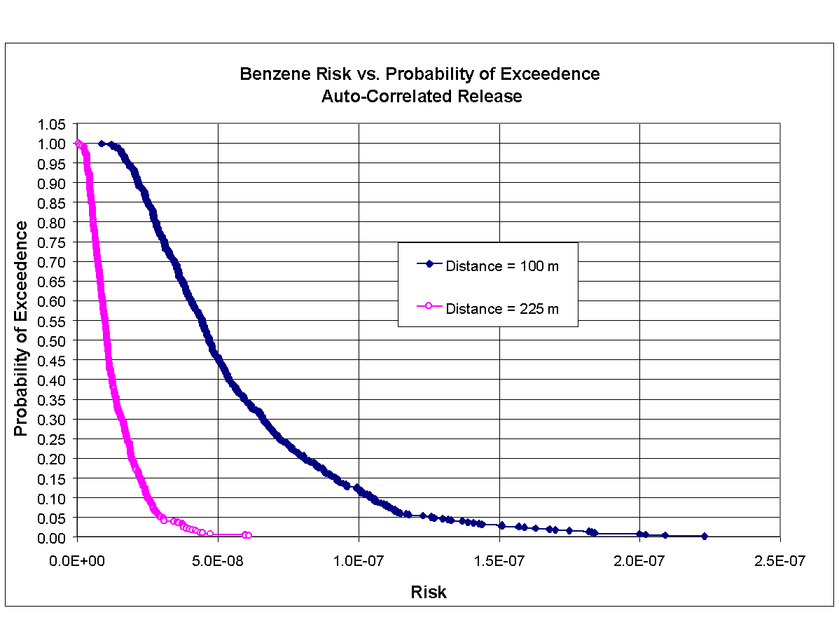
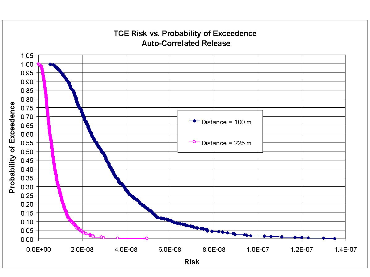
Figures 8.12 and 8.13 present the cumulative distribution function (CDF) curves that developed from the results of the Scenario 3 Monte Carlo analysis, corresponding to benzene and TCE, respectively, for distances of 100 and 225 m. These figures plot the probability of exceedence versus carcinogenic risk (i.e., excess cancer incidence). As can be seen in these figures, the probability of exceeding a risk of 10-6 is nearly zero for both constituents at both distances.
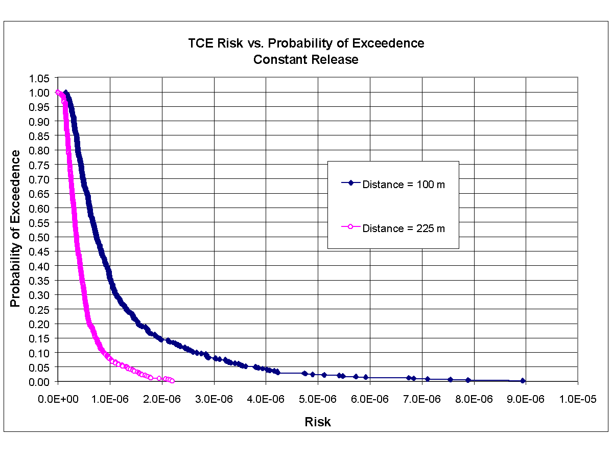
To demonstrate that conservatism has been built into the analysis, a probabilistic assessment associated with Scenario 2 (i.e., steady-state analysis) was also implemented. The values for stochastic parameters were assigned same value as those employed under Scenario 3, except for the emission rate. The emission rates for benzene and TCE were assumed to be constant at 6.16 m g /L and 16.16 m g/L, respectively, with the maximum and minimum values being set equal to twice and one-half of the mean. The standard deviation was set equal to one-third of the range, as it was in the previous Monte Carlo assessments. Figures 8.14 and 8.15 present CDF curves developed from the results of the Scenario 2 constant Monte Carlo analysis, corresponding to benzene and TCE, respectively, for distances of 100 and 225 m. These figures plot the probability of exceedence versus carcinogenic risk (i.e., excess cancer incidence). As can be seen in Figure 8.14 for benzene, there is a 5% probability of exceeding a risk of 3.7x10⁻⁶ and 1.2x10⁻⁶ at distances of 100 and 225 m, respectively. As can be seen in Figure 8.15 for TCE, there is a 5% probability of exceeding a risk of 3.8x10⁻⁶ and 1.2x10⁻⁶ at distances of 100 and 225 m, respectively.
Table 8.6. Stochastic Parameters in Comparative Assessment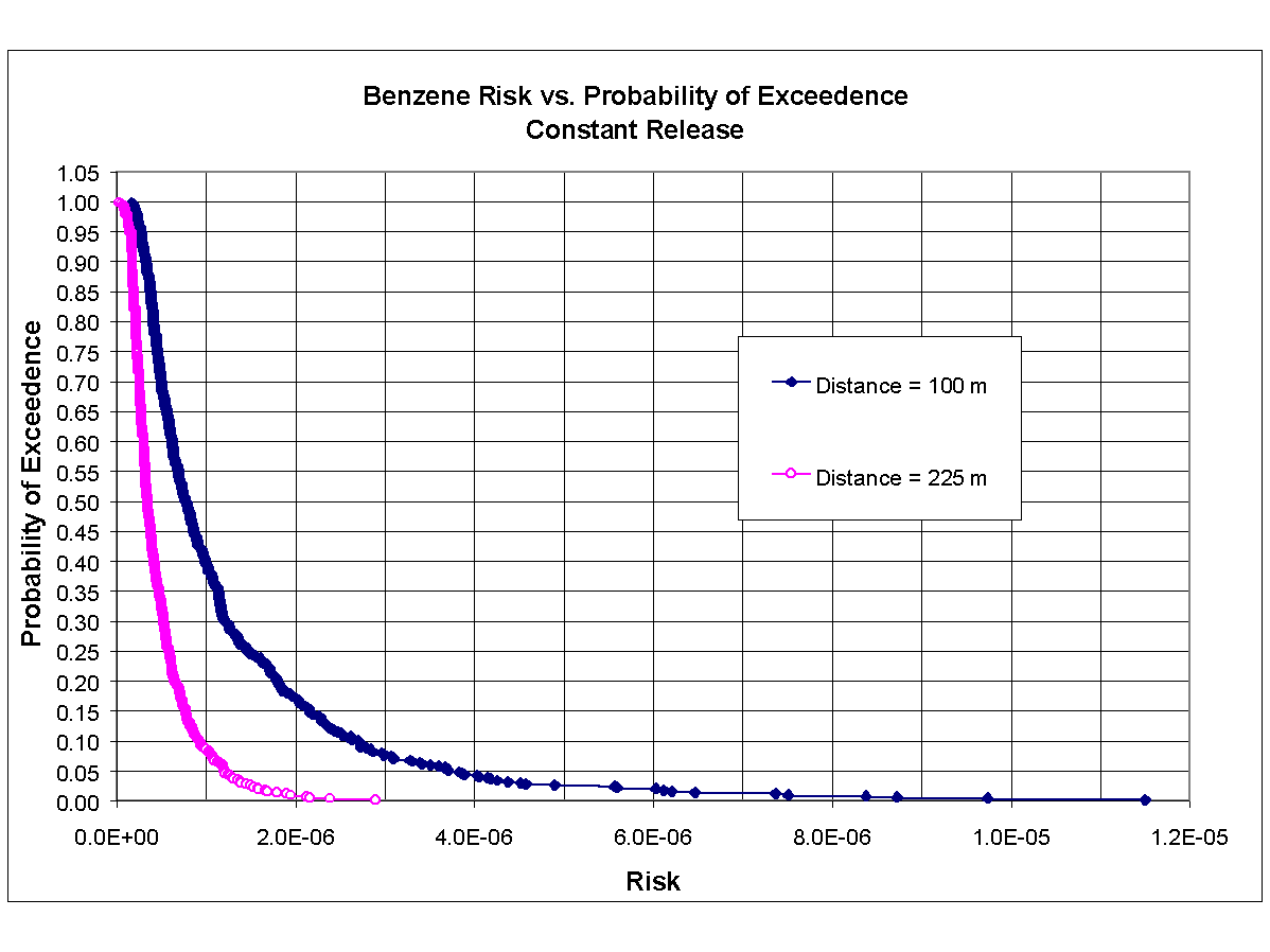
| Parameter | Distribution | Max. Value | Mean Value | Min. Value | Std. Dev. | Units |
| Benzene Flux at t = 0 yr | Normal | 0.565 | 0.282 | 0.141 | 0.141 | g/yr |
| TCE Flux at t = 0 yr | Normal | 1.386 | 0.693 | 0.347 | 0.347 | g/yr |
| Longitudinal Dispersivity (100 m)a,b | Normal | 2000 | 1000 | 500 | 500 | cm |
| Longitudinal Dispersivity (225 m)a,b | Normal | 4500 | 2250 | 1125 | 1125 | cm |
| Benzene Kd | Normal | 5 | 2.0 | 1 | 1.33 | mL/g |
| TCE Kd | Normal | 5 | 2.092 | 1 | 1.33 | mL/g |
|
aTransverse Dispersivity was computed by multiplying the Longitudinal Dispersivity by 0.165. bVertical Dispersivity was computed by multiplying the Longitudinal Dispersivity by 2.5E-3. |
||||||
9.0 References
APHA. 1986. Selected Physical and Chemical Standard Methods for Students. American Public Health Association, Port City Press, Baltimore, MD.
Buck, J. W., G. Whelan, J. G. Droppo, Jr., D. L. Strenge, K. J. Castleton, J. P. McDonald, C. Sato, and G. P. Streile. 1995. Multimedia Environmental Pollutant Assessment System (MEPAS©): Application Guidance -- Guidelines for Evaluating MEPAS© Input Parameters for Version 3.1. PNL-10395. Prepared for U.S. Department of Energy by Pacific Northwest Laboratory, Richland, Washington.
Codell, R. B., K. T. Key, and G. Whelan. 1982. Radionuclide Dispersion Analysis. NUREG-0868. Prepared by Pacific Northwest Laboratory for Nuclear Regulatory Commission, Washington, D.C.
Doctor, P.G., T.B. Miley, and C.E. Cowan. 1990. Multimedia Environmental Pollutant Assessment System (MEPAS©) Sensitivity Analysis of Computer Codes. PNL-7296, Pacific Northwest Laboratory, Richland, Washington.
EPA. 1989. Risk Assessment Guidance for Superfund Volume 1 Human Health Evaluation Manual (Part A). EPA/540/1-89/002, U.S. Environmental Protection Agency, Office of Emergency and Remedial Response, Washington, D.C.
Meyer, P.D., M.L. Rockhold, G.W. Gee. 1997. Uncertainty Analyses of Infiltration and Subsurface Flow and Transport for SDMP Sites. NUREG/CR-6565. PNNL-11705. U.S. Nuclear Regulatory Commission, Office of Nuclear Regulatory Research, Washington, DC.
USAF. 1993. Eielson Air Force Base, OU-2 Remedial Investigation/Feasibility Study, Remedial Investigation Report. Table 5.7, Eielson Air Force Base, 343rd Wing, Eielson, Alaska.
Whelan, G., K.J. Castleton, J.W. Buck, G.M. Gelston, B.L. Hoopes, M.A. Pelton, D.L. Strenge, and R.N. Kickert. 1997. Concepts of a Framework for Risk Analysis in Multimedia Environmental Systems (FRAMES). PNNL-11748. Pacific Northwest National Laboratory, Richland, Washington.
Whelan, G., J. W. Buck, D. L. Strenge, J. G. Droppo, Jr., B. L. Hoopes, and R. J. Aiken. 1992. "Overview of Multimedia Assessment Methodology MEPAS©." Haz. Waste Haz. Mat. 9(2):191-
Doctor P.G., T.B. Miley, C. E. Cowan. 1990. Multimedia Environmental Pollutant Assessment System (MEPAS©) Sensitivity Analysis of Computer Codes, PNL-7296, Pacific Northwest Laboratory, Richland, Washington.
Cochran, W.G. 1963. Sampling Statistics. 2nd ed. John Wiley and Sons, New York.
Doctor, P. G., E. A. Jacobson, and J. A. Buchanan. 1988. A Comparison of Uncertainty Analysis methods Using a Groundwater Flow Model. PNL-5649, Pacific Northwest Laboratory, Richland, Washington.
Iman, R. L., J. M. Davenport, and D.K. Zeigler. 1980. Latin Hypercube Sampling (Program User´s Guide). SAND79-1473, Sandia National Laboratories, Albuquerque, New Mexico.
Iman, R. L., and W. J. Conover. 1982. A Distribution-Free Approach to Reducing Rank Correlation Among Input Variables. Communications in Statistics B11(3):311-334.