
![]() Appendix A
Appendix A
A.1 Data Dictionary
A.2 Sensitivity Uncertainty
A.3 Model Considerations
A.4 Editors
A.5 Server Side
A.3 MODEL SPACE AND TIME CONSIDERATIONS
The ultimate intent is to propose a universal design for meeting protocols for linking disparate models and ensuring communication between environmental software products. The design is not intended to be parochial or inflexible but is intended to set the standard for allowing a number of different approaches to communicate within a framework. For example, if the requirement is to allow two models to seamlessly communicate, then the interface design between these two models should be such that data should seamlessly pass from one model to the next, irrespective of scale or resolution (within reason), and should not be model-dependent. These protocols are applicable, regardless of whether the models are on local or remote systems.
A.3.1 Model Connectivity
Model connectivity addresses the issues associated with ensuring the transparent linkage (i.e., how models communicate with each other) between models with different scale and resolution. Scale refers to the physical size and requirements of the problem (e.g., medium-specific, watershed, regional, and global). Resolution refers to the temporal- and spatial-mesh resolution associated with the assessment [i.e., requirements associated with the transfer of data at medium interfaces (i.e., boundary conditions)], designated as low (e.g., structured-value), medium (e.g., analytical), and high (e.g., numerical). For example, an analytical model, using mass flux across an infinite plane, should structure its output to be handled by another analytical model or numerical model containing a grid system. Any design should be general enough and structured to ensure that mass is conserved and that the linkage handles most types of traditional models.The responsibilities of the consuming module would include processing, mapping, and transforming the producing models output, as correlated to the Geo-Referencing system, to a standard format described by a Model Dictionary File. The consuming model would be charged with:
- recognizing and understanding the dataset corresponding to the Model Dictionary File
- mapping all spatially indexed parameters to the consuming models input requirements
- ensuring that the Geo-Reference system associated with the producing model and the assessment scenario is consistent with the consuming models Geo-Reference system.
The responsibilities of the producing module would include processing, mapping, and transforming the output to a standard format described by a Model Dictionary File. The producing model would be charged with:
- populating the Dataset corresponding to the Model Dictionary File
- mapping all spatially indexed parameters to meet system requirements
- mapping all temporally indexed parameters to meet system requirements
- ensuring that the Geo-Reference system associated with the producing model is consistent with the assessment scenario.
The boundary-condition data passing from one module to another will be handled through the Application Programming Interface Input/Output Dynamic Link Library. The linkage protocols and design will address the mapping of information between modules, specifically passing or calculating geo-spatial data, Geo-Reference coordinates, area-based polygons, and fractions of areas that overlap between producing and consuming model coordinate systems.
At the linkage or communication boundary, boundary information provided by the producing module would include the following:
- Spatially dependent, Geo-Referenced coordinates (i.e., vertices), describing points, lines, or polygons
- Associated with each set of vertices (e.g., polygon), will be spatially dependent, and constant or time-varying data.
The responsibilities of the consuming module would include processing, mapping, and transforming the producing models output, as described by the producing module's coordinate system, to the consuming model's coordinate system, which would involve mapping the producing model's spatially dependent, Geo-Referenced coordinates onto the consuming model's spatially dependent, Geo-Referenced coordinates and determining the fractions of areas that overlap. The mapping process will use the producing model's areas at the boundary that are projected onto the consuming model's boundary surface.
It is recognized that the consuming model may not have programs developed to perform the processing and mapping of and transformation associated with the producing model's output. Although not a responsibility of the system, the Application Programming Interface Input/Output Dynamically Link Library will provide a routine that:
- Calculates area-based polygons associated with producing and consuming model boundary surfaces, as defined by its spatially dependent, Geo-Referenced coordinates
- Maps the producing model polygons onto the consuming model polygons
- Calculates the fractions of the producing model polygon areas that overlap with each consuming model polygons
- Transforms the boundary conditions from the producing model's output to the consuming model's input by combining the producing model's output in an appropriate manner, so as to define the boundary conditions associated with each consuming model's boundary condition polygon.
In other words, if a consuming model needs assistance in transforming a producing model's output for consumption, a system program will be made available, which maps and assigns a producing model's output to all consuming models boundary-condition polygons. Based on this mapping, the consuming model would be charged with completing the mapping of the information associated with their polygons to their nodes, if required.
A.3.2 Geo-Referencing Considerations
The Model Dictionary Files contain information that allow for all spatially dependent boundary condition data to be referenced to a Geo-Reference system (i.e., x, y, z coordinates). The location aspect of the data is associated Geo-Referenced points, lines or polygons, as defined by their vertices. Tables A3.2.1 and A3.2.2 illustrate the Geo-Referencing scheme using Model Dictionary Files. Table A3.2.1 presents an example set of Model Dictionary Files for boundary condition polygon locations, and Table A3.2.2 presents an example set of Model Dictionary Files for time-varying chemical groundwater concentrations by boundary-condition polygons. These Geo-Referenced vertices allow for the mapping of the spatially distributed and dependent boundary condition data from the producing model boundary condition polygons to consuming model boundary condition polygons. This conversion is facilitated by an Application Programming Interface through a Dynamically Linked Library.A.3.3 Models with Spatial Boundary Conditions
Many models with spatial boundary conditions perform their boundary condition calculations at nodes, as opposed to the areas surrounding the nodes. Each node , though, represents a polygon that surrounds it. It is the polygon, and specifically the vertices of each polygon, which represents the basis for passing information between producing and consuming models.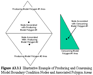 The nodes are represented by polygons, which, in turn, are described by their vertices portrayed within the model- and scenario-Geo-Referencing system (x, y, z coordinates). Tables A3.2.1 and A3.2.2 illustrate the metadata associated with the manner in which a model will describe and document the vertices of an area polygon. Figure A3.3.1 presents an illustrative example of producing and consuming model boundary condition nodes and associated polygon areas, whose corners represent polygon vertices.
For an analytical model, a rectangular plane traditionally defines the interface area with the vertices being defined at the four corners of the rectangle. For a numerical model containing a gridding system, multiple nodes and/or areas will be defined at the boundary interface. The producing model will be responsible for transforming its output to meet the boundary condition metadata requirements of the Model Dictionary Files, as illustrated in Tables A3.2.1 and A3.2.2. If the producing model provides its output by node, it will have to convert its node-based output to correspond to an area (i.e., polygon) representing each node. Either the model can do the conversion or the model can request help from the system, and the system will provide software to help in this conversion.
The Comprehensive Chemical Exposure Framework will assume that the boundary condition information is 1) associated with each polygon area, representing each boundary condition node, and 2) uniformly distributed across each polygon. 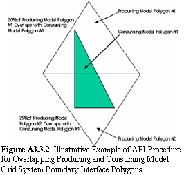 Figure A3.3.2 illustrates two areas associated with the boundary of a producing model (i.e., polygons #1 and #2), overlapping with one area associated with the boundary of a consuming model (i.e., polygon #1). When the producing model defines the output at a node, the producing model is responsible for transforming that nodal output into a form representing the area-based polygon. The consuming model has the responsibility to map the output results of each producing models polygons to the area-based polygons and corresponding nodal locations associated with the consuming models grid system. All interface mapping will be assumed to occur across a flat plane. If the gridding system boundary for one of the models is curvilinear, the producing models area, projected onto the consuming models surface, will be used in the mapping exercise.
If a consuming model does not have a mapping routine that transfers the producing models polygon-based output (e.g., time-varying mass flux and polygon vertices, which describe the area) to the appropriate and corresponding consuming models polygons, then the system will provide software to assist the consuming model in the mapping exercise. The consuming model can use this mapping software through the Application Programming Interface, or it can utilize its own mapping software. If system software is used, the Application Programming Interface will compute polygons around each node, defining the polygons by their Geo-Referenced vertices. The system assumes that the output at each node is associated with the area surrounding the node and that the output is uniformly distributed across the nodes assigned area. This assumption would be applicable for both producing and consuming models.
By utilizing the CCEF Application Programming Interface, a consistent procedure exists to develop the areas (i.e., polygons) associated with each producing or consuming models nodes. There are a number of methods for generating polygons (i.e., multiple-connected planar domains) to describe irregular computational grids (e.g., Thiessen Polygon Method, Voronoi Diagrams); the CCEF will use Voronoi Diagrams (Icking, 2001). Either module can invoke the Application Programming Interface to help it with the development of polygons. The extent of the areal planes associated with the producing and consuming models do not have to be identical. In other words, the sizes of the overlapping consuming and producing model planes could be different, as illustrated in Figures A3.3.1 and A3.3.2(above). The CCEF would then calculate the fraction of each producing polygon that overlaps with a consuming polygon.
When the producing and consuming model areas do not exactly overlap, the output, being transferred from the producing module to the consuming module, will be defined by the weighted-average associated with the overlapping areas (i.e., fraction of the producing model polygon overlapping with the consuming model polygon). In other words, the output assigned to the consuming modules nodal area will be defined by the output of the producing modules nodal areas, whose nodal areas overlap, weighted by aerial extent. The polygons for both the producing and consuming models are assumed to be convex, that is, the angles between vertices will not contain any interior angles that are greater than 180 degrees.
The transformation (i.e., mapping) of a producing models grid system onto a consuming models grid system area is illustrated in Figure A3.3.2 (above). In this illustrative example, the producing model has two polygons associated with it, while the consuming model (shaded area) has one. Approximately 20% of the producing model polygon #1 overlaps with the consuming model polygon #1, and the 35% of the producing model polygon #1 overlaps with the consuming model polygon #2. In effect, the information passing from the producing model's to the consuming models nodal area will be represented 20% and 35% of the output supplied by producing model polygons #1 and #2, respectively.
A.3.4 Models with Temporal Boundary Conditions
Each model, especially numerical models, calculate time stepping and have a nodal-spacing mesh that are consistent with their own model while ensuring numerical convergence and stability. Temporal considerations for linking models with disparate time-stepping requirements need to be independent of any model. To remove model-specific time stepping from dictating the manner in which models communicate, each of the models time-stepping requirements need to be accounted for when passing information between models.Each producing model will provide time-varying output corresponding with each producing models area-based polygons, which describe the boundary interface between models. The time-varying output from the producing model is a function of the time steps used in generating the time-varying curve. The system does not know if the time information between data-points on the mass flux rate curve is linear, constant, nonlinear, etc.; as such, each producing models time-varying curves will have their own time-stepping protocol for each parameter for each polygon. When the consuming model maps the producing models polygon output and transfers the information from the producing models gridding system to its own, the consuming model is responsible to account for the time-stepping system that the producing models provides. For example, if the producing model provides uneven time intervals with its output, but the consuming model requires even-incremented time steps, then the consuming model is responsible for ensuring the proper conversion.
For those consuming models that do not have a protocol for mapping producing model results into a form that they can recognize, the system Application Programming Interface provides software that can help in this mapping process. If the consuming model utilizes the system mapping protocol, then it is assumed that the consuming models time-varying input, which corresponds to a nodal polygon, is defined by the producing model's area-weighted output, whose producing models polygons overlap with the consuming models polygon. By passing area-weighted information, the system can transform the data from the producing models gridding system into a format that is consistent with the consuming models gridding system. The mapping procedure, using the system Application Programming Interface, is as follows:
- The system Application Programming Interface determines the fraction of the projection of the producing models polygon areas onto each consuming models polygons. For example, Figure A3.3.2 (above) illustrates the spatial mapping of two producing model polygons onto a consuming model polygon.
- The system Application Programming Interface multiplies each time-varying curve by their respective fractions.
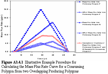 Figure A3.4.1, correlated with Figure A3.3.2, provides an example, which maps time-varying output from the two producing models polygons onto a corresponding consuming models polygon.
 - The system Application Programming Interface ensures that the time-stepping protocol associated with each producing models time-varying curves are consistently mapped, ensuring that each time step is accounted for, assuming linear interpolation, when necessary. If the system Application Programming Interface needs to combine the output from two producing model polygons, and the time-step intervals associated with each output is different, then the Application Programming Interface will linearly interpolate to ensure that the time steps for both time-varying curves have values corresponding to not only their own polygon time-steps, but also to the other polygon time steps. For example, if polygon #1 provides output every 10 years, and polygon #2 provides output every 5 years, then values will be assigned to polygon #2 corresponding to every five years, using linearly interpolation.
- The system Application Programming Interface summarizes the producing models area-weighed output to produce time-varying input for manipulation and consumption by the consuming model. For each point in time,
where
where fi represents the fraction of the producing models area that overlaps with the consuming models area, Ai represents the i-th producing models area that overlaps with the consuming models area, ATi represents the area in the i-th producing models polygon, "i" is the index on the i-th polygon in the producing models gridding system that overlaps with the area associated with the consuming models polygon, n is the total number of producing model polygons whose areas overlap the area associated with each corresponding consuming-model polygon, and j is the index on the j-th polygon in the consuming models gridding system.
Figures A3.3.2 and A3.4.1 (above) illustrate how a producing models output for two polygons can be transformed to produce input to the consuming models polygon. Figure A3.4.1 illustrates the mechanics of implementing Equations (1) and (2), as they relate to Figure A3.3.2. Five curves are presented in Figure A3.4.1: 1) two time-varying mass flux rate curves for the producing models polygons #1 and #2 (represented by solid squares and triangles, respectively), 2) two time-varying producing model curves, adjusted for the fraction of overlap between the producing and consuming model polygons (e.g., 20% and 35%) (represented by open squares and triangles, respectively), and 3) consuming models curve associated with its polygon (represented by open circles). Multiplying the aerial fractions times the corresponding polygon output and summing the results produces the input curve (i.e., open-circle curve in Figure A3.4.1 for the consuming model. The consuming model can then manipulate and transform this input curve to meet its model-specific input requirements.
A.3.5 Dynamic Simulation
Dynamic simulation refers to the ability of the system to allow for temporal dynamic feedback between models. Currently, the user has a choice between Plug & Play with no dynamic feedback or dynamic feedback where all of the models are "hard-wired" together with Plug & Play features. Under the design of the Comprehensive Chemical Exposure Framework, the Plug & Play feature would be combined with the temporal feedback feature. This could be done by allowing the upstream model to proceed with calculations until the temporal results are available and encompass a time step associated with the downstream model. The downstream model would then begin calculations until its temporal results are available and encompass the next time step of the downstream model. The procedure is repeated until all time steps for both models have been addressed. This approach is consistent with the design structure of the Application Programming Interface and Data Dictionary Files.