5.5 Mass Loss Expressions for Multiple Concurrent Loss Routes

     In general, first-order decay/degradation, leaching, wind suspension, water erosion, and volatilization could all be happening concurrently; and some type of remediation methodology could be implemented at some point during the simulation time. The multiple, concurrent processes can interact; which can cause the mathematical expression for a given term in Equation 5.56 to be different from what it would be if that process was the only one removing mass from the source zone. When processes occur simultaneously, the appropriate mathematical formulations are as follows.

     The mass flux term for loss from the source zone by decay/degradation is still given by the expression in Equation 5.57. This is true even for the scenario in which an ISS remediation methodology has been implemented. Recall that the conceptual model for this scenario assumes that a spatial gradient in concentration develops inside the waste form as contaminants diffuse out of it. However, it is true that



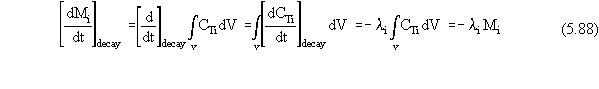
     which demonstrates that Equation 5.57 is still valid. However, for an ISS scenario, if decay products are also contaminants of interest, the mass of decay products produced by the decay term (Equation 5.57) for the parent contaminant is not added back into the mass of the source zone for consideration in subsequent time steps. The necessity of this restriction arises from the fact that the mass flux term for leaching from an ISS waste form is based on spatial concentration gradients and contaminant masses in the source zone at the initial time, rather than at the actual time. (This is different than the way the source-term release module handles the accumulation and subsequent loss of decay products of concern for other scenarios.)

     The term for leaching can take on one of several different forms depending on the particular scenario being simulated (e.g., whether a NAPL phase exists, whether a clean soil layer exists above the source zone, whether a remediation methodology has been implemented). In general form, the mass flux term for loss from the source zone by leaching is still given by Equation 5.60. When a NAPL phase exists in the source zone, the mass flux term for loss from the source zone by leaching is still calculated by Equation 5.60 directly, with the value of C_wicalculated form the phase partitioning theory described in Section 2.2.4, as before.

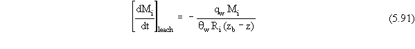
     When no NAPL phase exists in the source zone, the mass flux term for leaching may take on a number of forms. When no ISV or ISS remediation methodology has been implemented, consider that the aqueous concentration of the contaminant is given by Equation 2.7, and the volume of the source zone is given by Equation 5.69. Substituting Equations 2.7 and 5.69 into Equation 5.60, we obtain



     Now all that remains is to determine the correct way to express the thickness, h, of the source zone that appears in Equation 5.89. The position of the lower boundary of the source zone is constant in time. On the other hand, the position of the upper boundary of the source zone may be changing due to volatilization and/or wind suspension and water erosion. Firstly, consider a scenario where a clean layer of soil exists above the source zone initially. Depending on the relative rates of wind suspension, water erosion, and volatilization, it could be the case that the clean layer will always exist during the simulated time frame (and maybe even grow in thickness); or it could be the case that the clean layer will eventually be stripped away at some time during the simulated time frame. Secondly, consider a scenario where a clean layer of soil does not exist above the source zone initially. Again, depending on the relative rates of wind suspension, water erosion, and volatilization, a clean layer may never develop; or it may develop and always exist thereafter during the simulated time frame; or it may develop but eventually be stripped away at some time during the simulated time frame. As long as a clean layer is present, the process controlling the thickness of the source zone is volatilization. When no clean layer is present, the processes controlling the thickness of the source zone are wind suspension and/or water erosion. The criterion that must be used to determine which of these two regimes the system is in is a comparison between the position of the top of the source zone, z, and the position of the soil surface, which can be expressed as (S+E)t. Hence, the thickness of the source zone is given by



     Substituting the appropriate expression for h from Equation 5.90 into Equation 5.89, the mass flux term for loss from the source zone by leaching (when no NAPL phase is present) is given by



     for all times when a clean layer of soil exists above the source zone (i.e., when z (S+E)t), and is given by



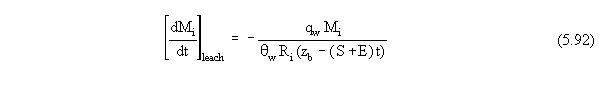
     for all times when a clean layer of soil does not exist above the source zone (i.e., when z (S+E)t).

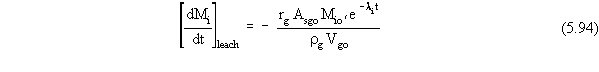
     For scenarios where an ISV remediation methodology has been implemented, the leaching term could still be given by the expression in Equation 5.64. However, as stated previously, expressions for the actual surface area and volume of the dissolving cracked glass as functions of time would be difficult to obtain in most instances. For ISV scenarios, wind suspension, water erosion, and volatilization mass fluxes are assumed to be zero because of the nature of the cracked glass waste form. This means that decay is the only other loss process occurring besides leaching. Therefore, the overall total concentration of a contaminant in the glass can be expressed as



     If we make the same idealizing assumption that was made when deriving Equation 5.66, the mass flux term for loss from the source zone by leaching for an ISV waste form is given by



     For scenarios where an ISS remediation methodology has been implemented, wind suspension, water erosion, and volatilization mass fluxes are assumed to be zero because of the nature of the ISS waste form. This is a good assumption for wind suspension and water erosion because the grouting of the source zone into a solid waste form prevents soil particles from being removed by these processes. However, in reality volatilization could still occur by outward diffusion through the grout, and then upward diffusion through a clean layer of soil, if one is present. Simulating volatilization in this scenario would require some type of coupled, two-region diffusion theory. It would also require some kind of conceptualization of how downwardly percolating vadose zone water impinging on the upper face of the waste form (i.e., the boundary between the two regions) and being channeled around the waste form, affects boundary conditions of the mathematical problem at the interface. Such theory for volatilization was not developed for the current version of the source-term release module.

     Recall that the conceptual model for leaching from an ISS waste form consists of diffusive movement of contaminants within the waste form to the outer boundary of the waste form, where they are lost to the vadose zone water that percolates past the faces of the waste form. The vadose zone water is assumed to move past the waste form fast enough that a zero concentration boundary condition applies for all contaminants at the faces of the waste form. The conceptualization leads to theory that predicts transient-state spatial gradients in concentration within the waste form. For any contaminant, i, the expression for mass flux out of the waste form developed from this theory (Equation 5.67 for the case where leaching is the only loss process) depends on the mass of contaminant i present in the waste form at the initial time (which was assumed to be spatially uniformly distributed within the waste for at that time). If contaminant i also undergoes decay/degradation, this same type of theoretical development can be used to obtain a similar expression for leaching loss mass flux (as a function of time) that accounts for the interaction of the decay/degradation process. Specifically, for all contaminants that are initially present in the source zone, the mass flux term for loss from the source zone by leaching (when decay/degradation also occurs) for an ISS waste form is given by



where

M_i,p is the total mass or activity of the p-th member of the decay/degradation chain that starts with contaminant i (g or Ci)
l_i,k is the first-order decay/degradation coefficient for the k-th member of the decay/degradation chain that starts with contaminant i (yr^-1)^.

     Note that for clarity later in the theoretical development, we have added an additional index to the subscripts of variables that depend on the particular contaminant species. The specific value '1' used for the second subscript indices p and k in Equation 5.95 denotes that this particular contaminant, i, was present in the source zone at the initial time (i.e., contaminant i is considered to be the first member of a possible decay/degradation chain of contaminants of concern). The quantity M_io",1 is the initial mass of contaminant i in the source zone. The quantity M_i,1 is the mass of contaminant i in the source zone at time t that originated from M_io",1, but that has been reduced from the value M_io",1 because of decay/degradation. The quantities l_i,1 and D_gi,1 are merely the first-order decay coefficient and effective diffusion coefficient in the waste form, respectively, for contaminant i. However, the added subscript index denotes that these are for a "parent" compound in a possible decay/degradation chain. Note also that Equation 5.95 is similar to Equation 5.67, except that an exponential decay factory for each contaminant initially present has been included. This factor, multiplied by the initial mass of the contaminant, is an expression of how the mass of contaminant i would have changed over time if no leaching loss would have occurred.

     If every contaminant i merely decayed/degraded into a nontoxic compound that was not of concern, Equation 5.95 is all that would be needed to predict the leaching of each contaminant of concern. However, if a contaminant initially present in the source zone decays/degrades into another contaminant, Equation 5.95 cannot account for this additional progeny mass during the simulation because only the initial mass (rather than the actual mass as time t) appears in the equation. In other words, there is no simple way to add contaminant mass back into the calculations for subsequent times (as we do with the solution of equations for other scenarios). One might be tempted to use the same type of equation as Equation 5.95, only reset the initial mass variable to the added mass, and reset the time variable to make t = 0 coincide with the time of production of the new mass. However, this is not a valid approach because the theory behind Equation 5.95 assumes that the mass is spatially uniformly distributed at the initial time, while what is really occurring in the source zone is that new mass is being produced nonuniformly over space because gradients in the contaminant that produced it already exist at time t.

     The source-term release module accounts for the leaching of progeny contaminants in the following way. For each contaminant i that is initially present in the source zone (as a "parent" contaminant), the module uses a set of equations to calculate the leaching losses of all progeny contaminants that were derived from the initial mass of contaminant i. Specifically, for all contaminants that are progeny of contaminant i, the mass flux term for loss from the source zone by leaching (when decay/degradation also occurs) for an ISS waste form is given by



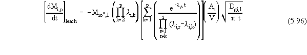
     Note that this equation is not an exact solution to the coupled contaminant diffusion problem because all contaminants may have their own unique effective diffusion coefficient in the waste form. Rather, Equation 5.96 contains the implicit assumption that all progeny contaminants have the same effective diffusion coefficient as their parent contaminant. In Equation 5.96, the product of the first three factors on the right-hand side of the equation is an expression of how the masses of progeny of contaminant i would have changed over time if no leaching loss would have occurred (i.e, it is the mass versus time function predicted by the Bateman equation [Bateman 1910]).

     Contaminants that are part of a decay/degradation chain of one of the contaminants present initially may actually be one of the initial contaminants, or may be the same as one of the contaminants in the decay/degradation chain of another initial contaminant. Therefore, after all of the mass fluxes denoted by Equations 5.95 and 5.96 are calculated, the ones that correspond to the same contaminant are added together to produce one set of leaching mass flux terms (i.e., this summation procedure is how the module accounts for the accumulation and subsequent loss of daughter products).

     When the soil is contaminated all the way up to the surface, the mass flux terms for loss from the source zone by wind suspension or water erosion are given by





     Note that Equations 5.97 and 5.98 are similar to the expressions in Equations 5.71 and 5.72 for individual loss pathways, except for the fact that the thickness of the source zone must now be expressed as a function of both of these particle loss processes. When there is a clean layer of soil at the surface, the mass flux terms for wind suspension and water erosion are zero.

     The appropriate mass flux terms for volatilization in scenarios where multiple contaminant loss processes are occurring concurrently were developed as follows. As was described above for the calculation of leaching loss mass flux terms, there may or may not be a clean layer present at any given time (depending on the relative rates of wind suspension, water erosion, and volatilization). When a clean layer is present, the mass flux term for contaminant loss from the source zone by volatilization is given by



     Note that Equation 5.99 is similar to Equation 5.73 (for the case where loss is by volatilization alone), except that the length of the diffusion path also depends on how much soil has been removed from the surface by wind suspension and water erosion. When a NAPL phase exists in the source zone, the vapor concentration in Equation 5.99 is calculated by the phase partitioning theory described in Section 2.2.4. When no NAPL phase exists in the source zone, C_vi, can be calculated by a simple phase partitioning relation, and the mass flux term is given by



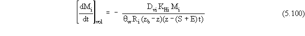
     When a clean layer is not present, or when it is so thin that Equation 5.99 would predict unreasonably high values, the mass flux term for volatilization at that time is again taken to be the bounding value calculated by Equation 5.86.

     Mass balance arguments (similar to those invoked when volatilization was the only process occurring) lead to the equation used by the module to compute the rate of recession of the upper boundary of the source zone, based on an individual contaminant, when a bounding value is not used for the volatilization flux term:



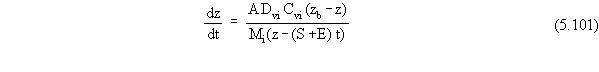
     When a NAPL phase exists in the source zone, the vapor concentration in Equation 5.101 is calculated by the phase partitioning theory described in Section 2.2.4. When no NAPL phase exists in the source zone, C_vi, can be calculated by a simple phase partitioning relation, and the rate of recession of the top boundary of the source zone, based on an individual contaminant, is given by



     When a bounding value is used for volatilization flux, the rate of recession of the top boundary of the source zone, based on an individual contaminant, is still given by Equation 5.87. As in the case where volatilization was the only loss process occurring, for contaminants that are components of the NAPL phase, Equation 5.80 is then used to calculate a single updated position of the top boundary of the source zone for all of the NAPL-phase components.

     As a final note, recall that the source-term release module tests to determine if a NAPL phase exists at the beginning of each time step. Based on the specific theory presented in this section for the contaminated vadose zone source zone, Equation 2.1 can be rewritten as



     for all times when a clean layer exists and



     for all times when a clean layer does not exist. Equations 5.103 and 5.104 are the test criteria that the module actually uses for contaminated vadose zone simulations.