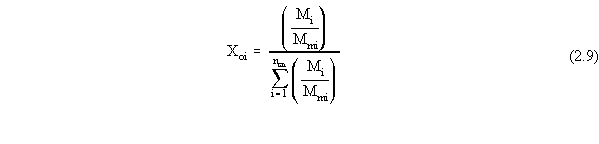
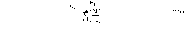
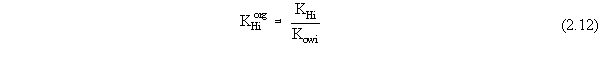
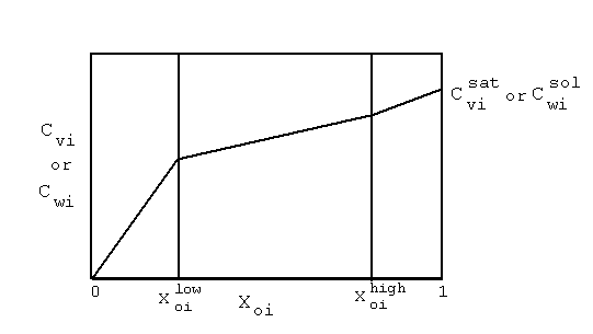
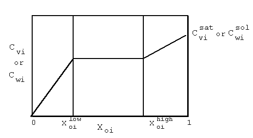
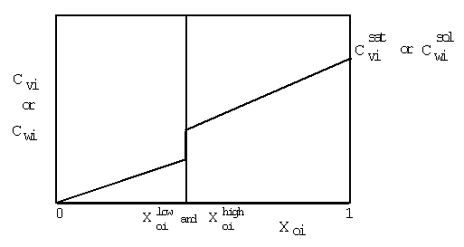
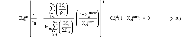
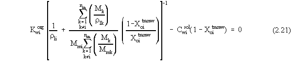
2.2.4  Partitioning Theory When a NAPL Phase Exists

 If a NAPL phase exists, two kinds of phase partitioning theory are used.  All contaminants that are not part of the NAPL phase (i.e., all contaminants with Henry's Law constants < 10^-7) are assumed to behave independently of one another, and are assumed to partition between aqueous, solid-sorbent, and vapor phases according to the theory presented in Section 2.2.3.  The partitioning behaviors of all contaminants that are part of the NAPL phase (i.e., Henry's Law constants 10^-7) are interdependent because the aqueous and vapor concentrations of each of these contaminants is controlled by the composition of the NAPL phase (which depends on all contaminants).

 An exact phase partitioning calculation (for the contaminants that can be a part of the NAPL phase) would require a simultaneous calculation of volumetric fluid contents (for water, air, and NAPL), and contaminant concentrations in all phases.  This type of full phase distribution model would require a complex and iterative algorithm (which could take a significant amount of time to run for each time step).  The current version of the source-term release module does not contain such a model; but, rather, makes the simplifying assumption that the composition of the NAPL phase is the same as it would be if all of the contaminant mass was in the NAPL phase.  It then further assumes that the volumetric water and air contents are equal to what they would be if there was no NAPL phase present.

For all contaminants that can be part of the NAPL phase, the source-term release module first calculates mole fractions and concentrations in the NAPL phase for each contaminant.  NAPL-phase mole fractions are calculated by



where

X_oi  is the mole fraction of contaminant i in the NAPL phase (unitless)
M_mi   is the molecular weight of contaminant i (g mol^-1)
n_cn  is the total number of constituents in the NAPL phase (unitless)
i  is the index on contaminant (unitless)

The NAPL-phase concentrations are calculated by




where

C_oi  is the concentration of contaminant iin the NAPL phase (g cm^-3 or Ci cm^-3)
r_li  is the density of contaminant i in the pure liquid form (g cm^-3).

Note that Equation 2.10 implicitly assumes that "volume-of-mixing" effects are negligible (i.e., when different liquids mix, the total mixed volume is equal to the sum of the individual separate volumes).

 For partitioning equilibrium between the NAPL and vapor phases, the module assumes that an analogue of the modified (i.e., dimensionless) Henry's Law is valid when the contaminant is present as a dilute constituent of the NAPL phase (i.e., when its concentration is sufficiently close to 0):




where    is the modified "Henry's Law" constant for contaminant i (concen./concen. basis) for partitioning between NAPL and vapor (unitless).

Note that the superscript "org" is used on the dimensionless Henry's constant to highlight the fact that this should be the value for partitioning from an organic liquid phase rather than from an aqueous phase (which is the usual value reported for Henry's Law constants).  This value, of course, depends on the exact composition of the organic liquid phase.  However, as a first approximation, this parameter can be estimated by




where     K_owi is the octanol-water partition coefficient for contaminant i (unitless).

The module assumes that Raoult's Law is valid when the contaminant is present as a primary constituent of the NAPL phase (i.e., when its mole fraction is sufficiently close to 1):




Figure 2.1 illustrates these "Henry's Law" and Raoult's Law type of relationships between vapor concentration and NAPL composition via the linear segments drawn below some low cutoff value and above some high cutoff value of NAPL-phase mole fraction.  For intermediate mole fractions, the vapor concentration will be somewhere in between the values at the cutoff mole fractions.  The source-term release module assumes that the vapor concentration in equilibrium with a NAPL phase containing the contaminant at an intermediate mole fraction can be calculated as a linear interpolation between the two values at the extremes of the "Henry's Law" and Raoult's Law regimes (as illustrated in Figure 2.1).  For partitioning equilibrium between the NAPL and aqueous phases, the module again assumes that an analogue of the modified (i.e., dimensionless) Henry's Law is valid when the contaminant is present as a dilute constituent of the NAPL phase (i.e., when its concentration is sufficiently close to 0):



where    is the analogue of the modified "Henry's Law" constant for contaminant i for partitioning between NAPL and aqueous phases (unitless).



Figure 2.1. Approximate Representation of Contaminant Vapor or Aqueous Concentration as a Function of NAPL-Phase Mole Fraction.  The region below  is in the "Henry's Law" regime; and the region above  is in the "Raoult's Law" regime.

The value of , of course, depends on the exact composition of the organic liquid phase.  However, as a first approximation, this parameter can be estimated by



The module also assumes that an analogue of Raoult's Law is valid (i.e., ideal solution behavior) when the contaminant is present as a primary constituent of the NAPL phase (i.e., when its mole fraction is sufficiently close to 1):



Because of the similarity between how the source-term release module conceptualizes equilibrium partitioning between a NAPL phase and a vapor or aqueous phase, Figure 2.1 also illustrates the "Henry's Law", "Raoult's Law", and intermediate region type of relationships used to calculate aqueous concentration from NAPL composition.

 Given the general forms of the phase equilibria curves in Figure 2.1, the NAPL-phase mole fractions at which the partitioning theory transitions from one regime to another must still be determined.  The source-term release module assumes that the high and low cutoff values of X_oi are chosen such that the ranges of mole fraction in which "Henry's Law" and "Raoult's Law" relationships are applicable are equal in length (i.e., - 0 = 1 - ).  They are also chosen such that the intermediate line is either strictly horizontal or strictly vertical (which depends on the relative magnitude of  or ). 

This means that the module assumes that the actual C_vi or C_wi versus X_oi curve looks like the curve in either Figure 2.2 or Figure 2.3.

 Determining transition mole fractions that give equally wide regions for the two limiting law regimes is accomplished by determining the mole fraction at which



for the NAPL/vapor equilibrium, and at which



for the NAPL/aqueous equilibrium.^(a)  Note that the "Henry's Law" types of relationships (Equations 2.17 and 2.18) are written in terms of NAPL-phase concentrations rather than mole fractions.  Therefore, before the transition mole fractions can be calculated, the concentration variables must be converted to mole fractions.  This conversion relationship is given by



Figure 2.2. Representation of Equilibrium Contaminant Partitioning Between NAPL and Vapor or Aqueous Concentration as a Function of NAPL-Phase Mole Fraction:  Implementation for the High or  Case.



Figure 2.3. Representation of Equilibrium Contaminant Partitioning Between NAPL and Vapor or Aqueous Concentration as a Function of NAPL-Phase Mole Fraction:  Implementation for the Low or  Case.



where    k is the index on the contaminants other than contaminant i (unitless).

Using Equation 2.19 to convert the concentration variables in Equations 2.17 and 2.18, and then moving everything to the left-hand sides of the equations, these two equations become





The source-term release module then uses a modified Newton-Raphson root-finding algorithm (Press et al. 1988) to solve Equations 2.20 and 2.21 for their respective lower transition mole fractions.  Once these lower transition mole fractions are determined, they are compared to 0.5.  If the lower transition mole fraction is < 0.5, a phase equilibrium curve shape like the one in Figure 2.2 is assumed.  If the lower transition mole fraction is 0.5, it is reset identically equal to 0.5 and a phase equilibrium curve shape like the one in Figure 2.3 is assumed.

 As stated in Section 2.2.3, the source-term release module ultimately needs values of the aqueous and vapor concentrations of the contaminants for the mass loss flux calculations.  When a NAPL phase is present, these are calculated as follows.  The contaminant's mole fraction in the NAPL phase is compared to the transition mole fractions (for vapor and aqueous equilibria) that have been previously calculated by the aforementioned method.  This determines which region of the phase equilibria curves (Figure 2.2 or 2.3) the contaminant falls into.  Based on that determination, the vapor concentration is calculated by using either Equation 2.11 or 2.13, or by setting it equal to the value at the transition mole fractions (if the actual mole fraction is in the intermediate region of a curve like that in Figure 2.2).  Similarly, the aqueous concentration is calculated by using either Equation 2.14 or 2.16, or by setting it equal to the value at the transition mole fractions (if the actual mole fraction is in the intermediate region of a curve like that in Figure 2.2

---

 

(a)	Note that in Equations 2.17 and 2.18, the variables with 'trans· ' in their superscript represent the low transition mole fractions or concentration. The high transition mole fractions are equal to one minus those values of the assumption of equally wide regions.